Visualising and exporting¶
How-to
At a glance
The docs visualisation helper, the in-memory
graph export (to_networkx / to_igraph for GraphML and, via NetworkX, GEXF),
and the native .tree / .clu formats written straight off the
Result.
A picture and a file¶
The partition lives in memory on the Result. Two ways to get
it out:
A picture: a network layout where every module gets a distinct colour.
Persistent output: files that other tools and scripts can open without re-running the algorithm.
Export formats¶
The export formats take different cuts through the same result:
to_networkx/to_igraphattach the module assignment, hierarchical path, and flow as node attributes inside the graph object, ready for GraphML or GEXF. Open the file in Gephi and colour nodes byinfomap_modulefor an interactive view of the same partition..treeis the full hierarchical tree. Every node appears with its path from the root (1:3means module 1, position 3 within it), its flow, its name, and its id. It is the most informative single-file summary..cluis the simplest format: node id, module, and flow per line. It loads with pandas or numpy in one line..ftreeis a.treeplus the intra-module link flows. It is what the Network Navigator reads to lay out and explore the modules.
Colour and export the karate club¶
The examples below use the Zachary karate club (34 people, 78 friendships).
Run Infomap¶
import networkx as nx
import infomap

g = nx.karate_club_graph()

result = infomap.run(g, two_level=True, seed=123, num_trials=10)
modules = result.modules()           # {node_id: module_id}

print(f"Nodes: {g.number_of_nodes()}, Edges: {g.number_of_edges()}")
print(f"Top-level modules: {result.num_top_modules}")
print(f"Codelength: {result.codelength:.4f} bits/step")
Nodes: 34, Edges: 78
Top-level modules: 3
Codelength: 4.0874 bits/step
Visualise the partition¶
The docs ship a small helper, draw_partition, that handles module colouring in
one call. It lives in the docs source tree and is importable in all executed
documentation pages.
import matplotlib.pyplot as plt
from myst_nb import glue

from docs_viz import draw_partition

# Marker area scales with flow, so a node's radius grows as the square root of
# how often the random walk visits it.
flow = {node.node_id: node.flow for node in result.nodes()}
fig = draw_partition(g, modules, flow=flow)
glue("fig-visualizing-and-exporting", fig, display=False)
plt.close(fig)
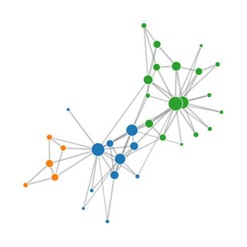
Fig. 8 The example network coloured by top-level module. The spring layout pulls tightly connected nodes together, so the colour boundaries line up with the visual gaps in the drawing.¶
draw_partition accepts several optional keyword arguments that are useful when
you adapt the pattern in your own code. seed fixes the layout, node_size sets
the base marker area, and flow scales each marker so its radius grows as the
square root of the node’s flow:
from docs_viz import draw_partition
import matplotlib.pyplot as plt

fig, axes = plt.subplots(1, 2, figsize=(10, 5))
draw_partition(g, modules, seed=7, ax=axes[0], node_size=200, flow=flow)
axes[0].set_title("seed=7")
draw_partition(g, modules, seed=99, ax=axes[1], flow=flow)
axes[1].set_title("seed=99")
fig.tight_layout()
For production figures, copy
interfaces/python/source/_ext/docs_viz.py and adapt it.
Export to GraphML and GEXF¶
For a single file bundling the network topology and the Infomap result,
infomap.to_networkx() (also available as
result.to_networkx()) builds a new
NetworkX graph from the result: nodes are the result’s (state) nodes, keyed by
state_id and carrying the Infomap node name plus the partition attributes,
and edges come from the partitioned network. NetworkX then writes it:
import os
import tempfile
from infomap import to_networkx

tmp = tempfile.mkdtemp()

annotated = to_networkx(result)   # new graph with infomap_module, infomap_path, flow, ...
graphml_path = os.path.join(tmp, "karate.graphml")
gexf_path = os.path.join(tmp, "karate.gexf")
nx.write_graphml(annotated, graphml_path)
nx.write_gexf(annotated, gexf_path)

print(f"GraphML: {os.path.getsize(graphml_path):,} bytes")
print(f"GEXF:    {os.path.getsize(gexf_path):,} bytes")
GraphML: 14,817 bytes
GEXF:    17,529 bytes
The exported graph carries these Infomap node attributes:
Attribute |
Value |
|---|---|
|
Top-level module id ( |
|
Colon-separated tree path ending in the node’s position within its module, e.g. |
|
One attribute per path component (the last is the node’s position within its final module) ( |
|
Stationary visit frequency ( |
GraphML and GEXF store the types alongside the values, so module ids and flows come back as numbers when the file is read — Gephi’s numeric colour scales and sorting work directly.
Because the graph is rebuilt from the result, your original graph’s node attributes are not carried over.
Open the GraphML file in Gephi, select Appearance → Nodes → Partition, and
choose infomap_module to colour the graph by community.
with open(graphml_path) as f:
    for line in f:
        if "infomap_module" in line:
            print(line.strip())
            break
<key id="d1" for="node" attr.name="infomap_module" attr.type="long" />
For igraph users, infomap.to_igraph() returns the same annotation on an
igraph.Graph.
Export to .tree and .clu¶
The Result carries the engine’s native text writers, so the
result from the run above writes the files directly — whatever built the
network. These formats feed the mapequation.org tools: .ftree opens in the Network
Navigator, and .tree/.clu load in the alluvial diagram generator and other
scripts.
tree_path = os.path.join(tmp, "karate.tree")   # full hierarchy with flow
clu_path = os.path.join(tmp, "karate.clu")      # flat node_id, module, flow
result.write_tree(tree_path)
result.write_clu(clu_path)

print(f"Wrote {os.path.getsize(tree_path):,} byte tree file")
print(f"Wrote {os.path.getsize(clu_path):,} byte clu file")
Wrote 1,037 byte tree file
Wrote 812 byte clu file
Read the first few data lines of each file to see the format:
def data_lines(path, n=6):
    """Return the first n non-comment lines of a file."""
    lines = []
    with open(path) as f:
        for line in f:
            if not line.startswith("#"):
                lines.append(line.rstrip())
            if len(lines) == n:
                break
    return lines

print("=== .tree (path  flow  name  node_id) ===")
for line in data_lines(tree_path):
    print(line)

print()
print("=== .clu  (node_id  module  flow) ===")
for line in data_lines(clu_path):
    print(line)
=== .tree (path  flow  name  node_id) ===
1:1 0.0909091 "0" 0
1:2 0.0627706 "1" 1
1:3 0.0714286 "2" 2
1:4 0.038961 "3" 3
1:5 0.0281385 "7" 7
1:6 0.00649351 "11" 11

=== .clu  (node_id  module  flow) ===
0 1 0.0909091
1 1 0.0627706
2 1 0.0714286
3 1 0.038961
7 1 0.0281385
11 1 0.00649351
The .tree path column uses colon-separated integers: 1:3 means the third
node listed inside top module 1. For hierarchical runs with more than two levels
you will see paths like 2:1:4. The .clu format uses the top-level module
number only; pass depth to write_clu to report a different level.
result.write_flow_tree writes a .ftree file that adds intra-module link
flows.
The find_communities shortcut¶
For a one-liner where you only need the NetworkX graph annotated in place,
infomap.find_communities() writes the module attribute directly onto the
graph and returns the community sets. Call a NetworkX writer yourself afterwards:
import networkx as nx
import infomap

g = nx.karate_club_graph()
communities = infomap.find_communities(
    g,
    module_attribute="infomap_module",
    seed=123, num_trials=10,
)
nx.write_graphml(g, "karate_infomap.graphml")
print(f"Found {len(communities)} communities")
Clean up¶
import shutil
shutil.rmtree(tmp)
print("Temp directory removed.")
Temp directory removed.
Pitfalls¶
Alluvial diagrams live on mapequation.org, not in this package. Write a
.ftreeand open it in the Network Navigator; the docs helper draws static module-coloured layouts only..clurecords the top level. Passdepthtowrite_clufor a deeper level;.tree/.ftreecarry the full hierarchy.to_networkxbuilds a new graph, not a copy of yours. Its nodes are the result’s (state) nodes keyed bystate_id, so your original graph is left untouched: its attributes are not carried into the export. Useinfomap.find_communities()orinfomap.io.export.annotate_networkx_graph()to annotate your own graph instead.
API pointers¶
Visualisation
draw_partition(the docs helper in_ext/docs_viz.py) draws a module-coloured spring layout and accepts an existingaxfor multi-panel figures.
In-memory graph export
infomap.to_networkx()builds a NetworkX graph from the result’s (state) nodes, annotated withinfomap_module,infomap_path, per-level ids, andflowas native Python types (module ids and level ids asint,flowasfloat,infomap_pathasstr); write it withnx.write_graphml/nx.write_gexf.infomap.to_igraph()builds the same graph as anigraph.Graph.infomap.io.export.write_graphml(),infomap.io.export.write_gexf(), andinfomap.io.export.annotate_networkx_graph()instead annotate your own graph with the partition. They accept either a post-run statefulInfomapor theResultit returned. (write_gexfsupports NetworkX only.)
Native engine formats (written by the Result)
infomap.Result.write_tree()writes a.treefile with the hierarchical path, flow, name, and node id for every node.infomap.Result.write_clu()writes a.cluflat table; passdepthto choose the level.infomap.Result.write_flow_tree()writes a.ftreefile that adds intra-module link flows.infomap.Result.write_csv(),infomap.Result.write_json(), andinfomap.Result.write_newick()write the same partition as CSV, JSON, and Newick for tooling that prefers those formats.infomap.Result.write()dispatches on the file extension (.tree,.ftree,.clu,.csv,.json,.nwk). The statefulInfomapkeeps the same writers through 2.x.
Going deeper¶
API reference gives the complete export signatures with every keyword argument.
The survey (§4) sets flow-based community detection against modularity-based methods [Smiljanić et al., 2026].
The
.ftreeformat adds intra-module link flows and is the basis for alluvial diagrams on mapequation.org.