Flow and random walks¶
Concept
At a glance
Infomap finds communities by asking where a random walker lingers. Flow is that walker’s stationary visit frequency, and modules are the regions that trap it.
What flow captures¶
Networks describe movement. Hyperlinks route web surfers between pages; readers follow citations to the papers that shape a field. To see the large-scale structure of that movement you need a currency that respects direction, weight, and how paths chain together.
Counting edges inside and outside groups misses something dynamic: the way a random walker entering a dense cluster tends to stay there for many steps before it escapes. That persistence is what defines a community in flow-based clustering: a module is a part of the network where flow lingers [Rosvall and Bergstrom, 2008].
The map equation, Infomap’s objective function, measures how compactly the walker’s trajectory can be described. To do that it needs to know how often the walker visits each node and how often it crosses module boundaries. Both come from flow.
The random walk¶
Picture a walker that starts at some node and, at each step, follows one of the outgoing edges at random. It spends more time in densely connected regions and now and then crosses into another. Track where it sits over a long run, and the fraction of time spent at each node is that node’s flow, its stationary visit frequency.
The modules are the regions where the walker stays for many steps before it moves on. Inside such a region the walker’s path is long and locally predictable, broken only by rare crossings. The next chapter turns those long stretches into a two-level code and defines the description length that Infomap minimises.
Directed networks need one more ingredient. A directed graph can have dangling nodes (no out-edges) or sink components the walker can never leave, so the walk fails to reach every node; it is not ergodic. The fix is teleportation: with small probability \(\tau\) (default 0.15, the conventional PageRank value) the walker teleports to another node instead of following an edge. That guarantees a unique stationary distribution, but the jumps add long-range links that blur module boundaries. Unrecorded teleportation, which leaves the jump steps out of the recorded trajectory, removes most of the blurring and makes the partition robust to the value of \(\tau\) [Lambiotte and Rosvall, 2012]. Infomap uses unrecorded teleportation by default for directed networks.
Flow as a stationary distribution¶
A directed, weighted network on \(n\) nodes defines a transition matrix \(T_{ij} = w_{ij} / w_j^{\text{out}}\), where \(w_{ij}\) is the edge weight from \(j\) to \(i\) and \(w_j^{\text{out}}\) is node \(j\)’s total out-weight. The stationary distribution \(\pi\) satisfies
and gives the fraction of time a long random walk spends at node \(i\). Infomap calls this the flow of node \(i\). High-flow nodes sit at the network’s convergence points; many paths run through them, so the walker visits them often.
With teleportation at rate \(\tau\) the effective transition is
and the unique stationary solution \(\pi\) exists for any \(\tau > 0\). (At a dangling node, with no out-links to follow, the walker teleports with probability one rather than at rate \(\tau\).)
Where the walker lands after a teleport is a modelling choice. The \(1/n\) term
above is the simplest: uniform teleportation to any node. By default Infomap
instead teleports to a random link (proportionally to its weight) and lands at
the link’s source, so a node receives teleporting walkers in proportion to its
out-strength, and the next recorded step is always a real link traversal. With
recorded teleportation (recorded_teleportation=True) the walker lands at the
link’s target instead, proportionally to in-strength.
These per-node flows \(\pi_i\), together with how often the walker crosses between candidate modules, are the inputs the map equation needs. The next chapter, The map equation, turns them into the quantity Infomap minimises.
Computing the flow
For an unweighted undirected network the transition matrix is \(T_{ij} = A_{ij}/k_j\) where \(k_j\) is the degree of node \(j\), and the stationary distribution is \(\pi_i = k_i / (2|E|)\), proportional to degree. For a weighted directed network \(\pi\) is the leading right eigenvector of \(T\), which the power method computes iteratively.
For directed networks with teleportation, Infomap first computes \(\pi\) for the recorded walk (including teleportation steps), then re-weights it to count only link-traversal steps (the unrecorded scheme), so teleportation does not inflate the flow across module boundaries. See [Lambiotte and Rosvall, 2012] for the formal derivation.
Two cycles joined by a one-way bridge¶
The example below builds a tiny directed network by hand: two tight 3-cycles connected by a single bridge edge.
import networkx as nx
import infomap

# Two directed 3-cycles: A = {0,1,2} and B = {3,4,5}
G = nx.DiGraph()
G.add_edges_from([(0, 1), (1, 2), (2, 0)])   # cycle A
G.add_edges_from([(3, 4), (4, 5), (5, 3)])   # cycle B
G.add_edge(2, 3)                              # bridge: A leaks into B

print("Nodes:", list(G.nodes()))
print("Edges:", list(G.edges()))
Nodes: [0, 1, 2, 3, 4, 5]
Edges: [(0, 1), (1, 2), (2, 0), (2, 3), (3, 4), (4, 5), (5, 3)]
# Run Infomap on the directed network
result = infomap.run(G, directed=True, seed=123, num_trials=10)

# Read per-node flow (stationary visit frequency) and module assignments
flow    = {node.node_id: node.flow       for node in result.nodes()}
modules = {node.node_id: node.module_id  for node in result.nodes()}

print(f"Modules found : {result.num_top_modules}")
print(f"Codelength    : {result.codelength:.4f} bits/step")
print()
print(f"{'Node':>5}  {'Cycle':>7}  {'Module':>8}  {'Flow':>8}")
print(f"{'----':>5}  {'-----':>7}  {'------':>8}  {'------':>8}")
labels = {0: 'A', 1: 'A', 2: 'A', 3: 'B', 4: 'B', 5: 'B'}
for nid in sorted(flow):
    print(f"{nid:>5}  {labels[nid]:>7}  {modules[nid]:>8}  {flow[nid]:>8.4f}")
Modules found : 2
Codelength    : 1.7731 bits/step

 Node    Cycle    Module      Flow
 ----    -----    ------    ------
    0        A         1    0.0552
    1        A         1    0.0684
    2        A         1    0.0796
    3        B         2    0.2860
    4        B         2    0.2645
    5        B         2    0.2463
Nodes in cycle B carry higher flow than nodes in cycle A, even though the two
cycles have the same topology. The bridge 2 → 3 makes the difference: the
walker can drift from A into B but has no edge back. Teleportation is the only
return route, so cycle A collects fewer link-following visits and its flow stays
low. Infomap still puts each cycle in its own module, because each one is tight
relative to its links to the outside.
import matplotlib.pyplot as plt
from myst_nb import glue

from docs_viz import draw_partition

fig = draw_partition(G, modules, flow=flow)
glue("fig-flow-and-random-walks", fig, display=False)
plt.close(fig)
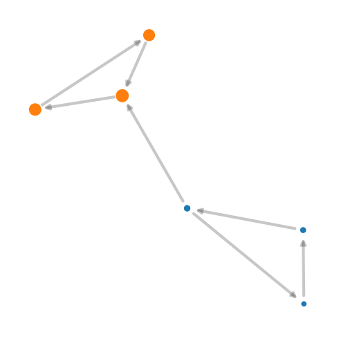
Fig. 1 A small network coloured by module. A random walker stays inside one colour for long stretches and crosses to the other only occasionally; those persistent visits are the flow the map equation compresses.¶
Teleportation and directed ergodicity
This example needs teleportation: without it a directed walk can get stuck in cycle B and never return to A, since no edge leaves B. Teleportation at rate \(\tau = 0.15\) restores ergodicity so every node stays reachable.
API pointers¶
infomap.run() is the entry point — pass directed=True for the directed
flow model with unrecorded teleportation — and returns a
Result; build non-default or programmatic input with
from_networkx() and add_link().
The result’s flow-bearing accessors (nodes(),
to_dataframe(), codelength) are
covered in Reading the result.
Going deeper¶
Source paper for flow-based community detection [Rosvall and Bergstrom, 2008]; teleportation in directed networks is developed in [Lambiotte and Rosvall, 2012].
The survey (§2–3) gives the broader treatment [Smiljanić et al., 2026], and the survey companion notebooks demonstrate flow on larger real-world networks.