Memory and state networks

Flow model

At a glance

When where flow goes next depends on where it came from, you need a memory network: state nodes encode the context, and the map equation on state nodes reveals overlapping communities that a first-order model cannot see.

Flow with memory

The standard map equation models a memoryless random walk: at every node the walker continues proportional to link weights, regardless of how it got there (see The map equation). In many real systems the dynamics carry memory: where flow goes next depends on where it has been.

Consider air passengers. A traveller arriving at Chicago from Seattle behaves differently from one arriving from New York: the Seattle traveller tends to return to Seattle, the New York traveller to New York. A standard network model, which sees only “a traveller at Chicago,” cannot capture that distinction. The same memory effect, where the path already taken constrains the next step, appears in citation patterns and patient transfers [Rosvall et al., 2014].

Ignoring this memory distorts community structure in two related ways. First, it makes modules look larger and less specific, because flow that is actually channelled by history appears to leak freely across boundaries. Second, it hides overlapping communities. In a second-order model, a multidisciplinary journal such as PNAS belongs simultaneously to several research communities depending on where a citation arrives from; a first-order model assigns it to a single module.

Splitting a node by its history

The core idea is to split each physical location into multiple state nodes, one for each relevant piece of context. In a second-order model the context is the previously visited node, so each directed edge \(i \to j\) in the original network becomes a state node at \(j\) that represents the history “arrived from \(i\).”

Think of a city intersection where two different streams of traffic pass through. One stream enters from the west and exits to the east, passing straight through. Another enters from the south and exits back to the south, a local detour. Model the intersection at first order and it appears in one community. Model the actual pathways and the two streams belong to different communities, with the intersection overlapping between them.

Infomap handles this with the physical node / state node distinction (see State nodes and higher-order flow for the general mechanism). State nodes carry the dynamics: they have links and stationary visit rates. Physical nodes represent the real objects you care about: they aggregate all their state nodes. The map equation encodes flow at the state-node level but names physical nodes in its codebook, so it correctly records a physical node whose state nodes land in different modules as overlapping [Edler et al., 2017].

Memory as a state-node network

A standard first-order network has physical nodes \(i\) and transition probabilities \(P_{ij} = w_{ij}/w_i\). In a second-order model, the walker’s next step depends on both the current node \(j\) and the previously visited node \(i\). We encode this as a state node \(\overrightarrow{ij}\) at physical node \(j\). The transition probabilities become

\[ P\!\left(\overrightarrow{ij} \to \overrightarrow{jk}\right) = \frac{w_{\overrightarrow{ij} \to \overrightarrow{jk}}} {\sum_l w_{\overrightarrow{ij} \to \overrightarrow{jl}}} \]

This is a first-order Markov chain on the expanded state-node graph, so Infomap’s standard machinery applies unchanged. The stationary visit rate of physical node \(k\) is the sum over all its state nodes:

\[ \pi_k = \sum_{\overrightarrow{jk}} \pi_{\overrightarrow{jk}} \]

When multiple state nodes of the same physical node land in the same module, the map equation aggregates their visit rates into a single codebook entry for that physical node. A physical node whose state nodes are split across modules is therefore assigned to multiple modules; overlapping community membership arises from the state-node formalism [Edler et al., 2017].

You do not have to commit to a full second-order model. The sparse memory network framework [Persson et al., 2016] lets you lump state nodes with similar outlink distributions, by minimising the entropy-rate loss, producing a variable-order model that fits the data efficiently without the exponential blowup of a fixed higher-order model.

State-node map equation

For a partition \(\mathsf{M}\) of state nodes into modules, the two-level map equation is

\[ L(\mathsf{M}) = q_{\curvearrowright} H(\mathcal{Q}) + \sum_{m=1}^{M} p^{\circlearrowright}_m H(\mathcal{P}_m) \]

The within-module codebook entropy \(H(\mathcal{P}_m)\) ranges over physical nodes, not state nodes:

\[ H(\mathcal{P}_m) = -\frac{q_{m\curvearrowright}}{p^{\circlearrowright}_m} \log\frac{q_{m\curvearrowright}}{p^{\circlearrowright}_m} -\sum_{i \in \mathsf{M}_m} \frac{\pi_{i \cap m}}{p^{\circlearrowright}_m} \log\frac{\pi_{i \cap m}}{p^{\circlearrowright}_m} \]

where \(\pi_{i \cap m} = \sum_{\alpha_i \in \mathsf{M}_m} \pi_{\alpha_i}\) aggregates all state nodes of physical node \(i\) that are assigned to module \(m\). This aggregation is what enables overlapping physical-node membership: state nodes of the same physical node in different modules each contribute to separate codebook entries; see [Edler et al., 2017], §3.2.

The exit rate from module \(m\) is

\[\begin{split} q_{m\curvearrowright} = \sum_{\substack{\alpha_i \in \mathsf{M}_m \\ \beta_j \notin \mathsf{M}_m}} \pi_{\alpha_i} P_{\alpha_i \beta_j} \end{split}\]

These expressions reduce to the standard first-order map equation when each physical node has exactly one state node [Rosvall and Bergstrom, 2008].

Node i, visited in two contexts

The bundled states() network makes the memory effect concrete. Five physical nodes i, j, k, l, m carry the flow, and node i is visited in two different contexts:

• arriving from the j–k side, flow tends to continue back into j and k;

• arriving from the l–m side, it tends to continue back into l and m.

A memoryless walker cannot tell the two apart: at i it mixes both streams and the distinction is lost. A memory model splits i into two state nodes, one per context, so each keeps its own onward flow, and i ends up in both communities at once. This is the same bridging role node i plays in the multilayer example, reached through memory rather than layers.

First order: one blurred community

Start with the memoryless baseline. Aggregate the two contexts of i into a single node and run standard, first-order flow.

import infomap
import networkx as nx
from infomap import run
from docs_viz import draw_partition

# Physical network: i links to both pairs; {j,k} and {l,m} are the two groups.
g = nx.DiGraph()
g.add_weighted_edges_from([
    ("i", "j", 1.0), ("i", "k", 1.0), ("i", "l", 1.0), ("i", "m", 1.0),
    ("j", "i", 1.0), ("j", "k", 1.0), ("k", "i", 1.0), ("k", "j", 1.0),
    ("l", "i", 1.0), ("l", "m", 1.0), ("m", "i", 1.0), ("m", "l", 1.0),
])

result_first = run(g, two_level=True, directed=True, seed=123, num_trials=20, silent=True)
print(f"First-order modules: {result_first.num_top_modules}")
print(f"Codelength         : {result_first.codelength:.4f} bits")

assert result_first.num_top_modules == 1

First-order modules: 1
Codelength         : 2.2516 bits

With no memory the walker at i continues to j, k, l, m with equal probability, so flow leaks freely between the two pairs. Infomap finds a single module: the structure is in the wiring, but not in the memoryless flow.

Second order: i splits, communities overlap

Now the state network. The bundled states() loader carries the two contexts of i as two state nodes, with directed, weighted links (it comes pre-configured for directed flow).

result = run(infomap.datasets.states(), num_trials=20, seed=123, silent=True)

print(f"State nodes  : {len(list(result.nodes(states=True)))}")
print(f"Modules found: {result.num_top_modules}")
print(f"Codelength   : {result.codelength:.4f} bits")

# Two communities, at a lower codelength than the first-order run.
assert result.num_top_modules == 2

State nodes  : 6
Modules found: 2
Codelength   : 2.0114 bits

Two modules, and a lower codelength than the first-order run: the memory model describes the flow more efficiently and recovers the two groups the aggregate hid.

Read the overlap

Each physical node has one entry per state node in result.nodes(states=True). Group by node_id to find the physical node that lands in more than one module. Each state node exposes .node_id (the physical node it belongs to), .state_id, and .module_id.

from collections import defaultdict

name = {1: "i", 2: "j", 3: "k", 4: "l", 5: "m"}
phys_to_modules = defaultdict(set)
for node in result.nodes(states=True):
    phys_to_modules[node.node_id].add(node.module_id)

for pid, mods in sorted(phys_to_modules.items()):
    tag = "  ← overlap" if len(mods) > 1 else ""
    print(f"  {name[pid]}: modules {sorted(mods)}{tag}")

  i: modules [1, 2]  ← overlap
  j: modules [1]
  k: modules [1]
  l: modules [2]
  m: modules [2]

Physical node i carries two state nodes that land in different modules, so it belongs to both communities; j, k, l, m each sit in one. Overlapping membership falls straight out of the state-node formalism.

Visualise

Draw the state network directly. The two state nodes of i sit side by side in the centre, ringed together as the one physical node they share; each takes the colour of its own module, so the overlap is visible at a glance.

import matplotlib.pyplot as plt
from matplotlib.patches import Ellipse
from myst_nb import glue

# State-level links keyed by state id (the *States file); states 1 and 4 are
# both physical node i.
state_links = [
    (1, 2, 0.8), (1, 3, 0.8), (1, 5, 0.2), (1, 6, 0.2),
    (2, 1, 1.0), (2, 3, 1.0), (3, 1, 1.0), (3, 2, 1.0),
    (4, 5, 0.8), (4, 6, 0.8), (4, 2, 0.2), (4, 3, 0.2),
    (5, 4, 1.0), (5, 6, 1.0), (6, 4, 1.0), (6, 5, 1.0),
]
state_phys = {1: "i", 2: "j", 3: "k", 4: "i", 5: "l", 6: "m"}
state_module = {n.state_id: n.module_id for n in result.nodes(states=True)}

G = nx.DiGraph()
G.add_weighted_edges_from(state_links)

# Two triangles, with i's two state nodes centred so the split reads clearly.
pos = {2: (-1.7, 0.9), 3: (-1.7, -0.9), 1: (-0.5, 0.0),
       5: (1.7, 0.9), 6: (1.7, -0.9), 4: (0.5, 0.0)}

fig, ax = plt.subplots(figsize=(6.0, 4.4))
draw_partition(G, state_module, ax=ax, pos=pos, node_size=650)
nx.draw_networkx_labels(G, pos, labels=state_phys, ax=ax, font_size=11, font_color="white")
ax.add_patch(Ellipse((0.0, 0.0), 2.0, 1.15, fill=False, ls=(0, (4, 3)), ec="0.35", lw=1.3))
ax.annotate("one physical node i,\ntwo state nodes", (0.0, -0.72),
            ha="center", va="top", fontsize=8.5, color="0.35")
ax.set_xlim(-2.4, 2.4)
ax.set_ylim(-1.7, 1.4)
glue("fig-memory-and-state", fig, display=False)
plt.close(fig)

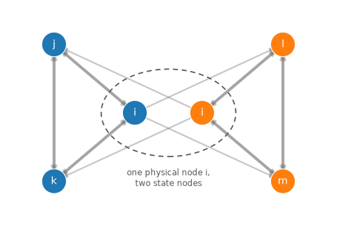
Fig. 9 The state network of the states() example. Physical node i appears as two state nodes (centre), one in each community; j, k join i’s first context and l, m its second. Colour shows the module; the dashed ring marks the two state nodes that are the same physical node.

Contrast

Node	First order	Second order
i	one merged module	both communities (overlap)
j, k	one merged module	with i’s first context
l, m	one merged module	with i’s second context

The first-order model blurs the two streams through i into a single community. The second-order model keeps them apart and lets i belong to both.

Options

Unlike the relax-rate multilayer model, the second-order model adds no dedicated engine flag on infomap.run(): it is defined structurally by the state nodes you declare on the Network. The knobs that shape and read a state network are:

Option	Where	Effect
add_state_node(state_id, node_id)	infomap.Network.add_state_node()	Declare one state node (a context) on a physical node
add_state_nodes(state_nodes)	infomap.Network.add_state_nodes()	Declare many state nodes at once
directed	infomap.run()	Follow link direction; a bare Network defaults to undirected flow, unlike the DiGraph route, which enables it automatically
states=True	infomap.Result.modules(), infomap.Result.nodes()	Return state-node assignments; required on higher-order networks, where states=False raises

API pointers

Declaring state nodes

net = Network()
net.add_state_node(state_id, node_id)

Creates a state node with a unique integer state_id mapped to the physical node node_id. If the physical node does not yet exist, add_state_node creates it. Use infomap.Network.set_name() afterwards for a human-readable label.

Adding state-level links

net.add_link(source_id, target_id, weight=1.0)

Links connect state nodes, not physical nodes. The same add_link serves both first-order and higher-order networks; in a state-node network source_id and target_id refer to state node ids.

Querying results

result = run(net)
result.have_memory                            # True when state nodes were added

# For memory networks, pass states=True
state_modules = result.modules(states=True)   # {state_id: module_id}

# Group state nodes by their physical node to find overlap
for node in result.nodes(states=True):
    node.node_id    # physical node id
    node.state_id   # state node id
    node.module_id  # module assignment for this state node
    node.flow       # state-node visit frequency

Because a physical node has one entry per state node in result.nodes(states=True), collecting all its module assignments requires grouping by node_id, as shown in the worked example.

Going deeper

• Source paper for memory networks [Rosvall et al., 2014]; sparse Markov chains for memory flows [Persson et al., 2016]; the Infomap implementation of higher-order flows [Edler et al., 2017].

• The survey (§5.1) covers higher-order and memory flows [Smiljanić et al., 2026]. Its companion notebook, examples/notebooks/5.1 Memory Networks.ipynb, works the *States file format and the add_state_node API on a small journal-citation example.