Reading the result

How-to

At a glance

infomap.run returns an immutable Result: summary statistics as properties, per-node assignments through modules() and nodes(), and tabular output through to_dataframe().

What the Result holds

A Result holds more than labels. Each node carries a flow value, the share of the random walk that visits it. The hierarchical tree records nested modules that a flat assignment vector cannot.

Three layers of detail

Think of the Result as three concentric layers of detail.

The outermost layer is a handful of scalars: codelength, number of top modules, number of levels. They answer “did it find something?” without access to individual nodes, and are cheap to inspect, log, and compare across runs.

The middle layer is the partition itself, a mapping from node id to module id. result.modules() returns it as a plain dict, {node_id: module_id}. Anything that expects a node-colouring can consume it directly.

The inner layer is per-node flow. Each node’s flow records the stationary probability of a random walk visiting it under the best partition. High-flow nodes are influential hubs; low-flow nodes are peripheral. This layer lets you rank nodes within a module or build flow-weighted summaries.

result.to_dataframe() materialises all three layers into one tabular object you can filter, group, merge, and export.

Why more than one trial

The Result reports the best (lowest-codelength) partition across the num_trials independent searches. One run is fine for exploration, but a single trial can settle in a local minimum, so results you publish or act on warrant more. See Running Infomap for why and the full num_trials rule of thumb. The rest of this chapter is about reading and comparing the partition you get back.

The solution landscape and degeneracy

Even for networks with clear community structure, Infomap produces a cloud of near-optimal partitions with similar codelengths but meaningfully different node assignments [Calatayud et al., 2019]. The variance of that cloud grows as community structure weakens (higher mixing parameter \(\mu\) in LFR benchmarks). For networks with \(\mu \le 0.2\), 50 trials are usually enough for the solution landscape to be “complete”, so further trials rarely reveal a different partition. Noisier networks can need 200 to 1000 trials. If you need to characterise the degeneracy rather than just find the best partition, consider the dedicated solution-landscape tooling.

Reading a karate-club result

The examples below use the Zachary karate club graph, a 34-node network with well-known community structure.

Run Infomap

import networkx as nx
import infomap
import pandas as pd

g = nx.karate_club_graph()

result = infomap.run(g, two_level=True, seed=123, num_trials=10)

The Result object

A Result is an immutable snapshot of one run. run() captures the scalar metrics when it returns. The Result materialises node-level collections lazily on first access and then caches them. The surface follows one convention:

• Read intrinsic results as properties — the scalar metrics (result.codelength, result.num_top_modules) and the fixed label and per-trial tables (result.names, result.state_names, result.codelengths). There is nothing to choose, so you read them like attributes, without parentheses.

• Call a method to slice, walk, or convert the partition — either you pass a view (result.modules(level=1), result.nodes(states=True), result.effective_num_modules(level)) or you ask for a built structure (result.summary(), result.to_dataframe()). The two canonical levels of effective_num_modules are also exposed as the result.effective_num_top_modules / result.effective_num_leaf_modules properties.

Reading a collection-valued property like result.names with parentheses raises a plain TypeError ('dict' object is not callable); drop them.

A Result from an earlier run of a reused stateful Infomap raises if you read its node data after a later run(). The eagerly captured scalar properties stay readable. The lazily computed effective_num_top_modules and effective_num_leaf_modules properties, and the effective_num_modules(level) method, stay readable only if you read them at least once before the re-run.

Summary statistics

The most useful summary properties are available immediately:

print(f"Codelength:          {result.codelength:.4f} bits/step")
print(f"One-level baseline:  {result.one_level_codelength:.4f} bits/step")
print(f"Compression gain:    {result.relative_codelength_savings * 100:.1f}%")
print(f"Top-level modules:   {result.num_top_modules}")
print(f"Hierarchy levels:    {result.num_levels}")

Codelength:          4.0874 bits/step
One-level baseline:  4.6340 bits/step
Compression gain:    11.8%
Top-level modules:   3
Hierarchy levels:    2

result.codelength is the map equation value \(L(\mathsf{M}^*)\) for the best partition found. result.one_level_codelength is the cost with all nodes in a single module, the natural baseline for judging how much structure Infomap found. result.relative_codelength_savings gives the fractional gap between the two; a larger number means stronger, more compressible community structure.

result.num_top_modules is the number of top-level modules. result.num_levels is the depth of the hierarchical tree (its deepest branch, on a ragged tree); a value of 2 means one level of modules above the leaves, the standard two-level result.

Recording what produced a result

result.provenance() returns, as a plain dict, the same record the engine writes into the .tree / .clu headers, the JSON tree and --manifest-json: the engine version, the effective seed and trial counts, the canonical configuration with its fingerprint, and the identity (path, size, mtime and a whole-content hash) of every file the run read. A network built in memory has no input identity, so result.provenance()["input"] is None then; the configuration and seed are always present.

record = result.provenance()
print(f"seed:        {record['seed']}")
print(f"config hash: {record['configFingerprint']}")
print(f"input:       {record['input']}")

seed:        123
config hash: 3432d148f835dde2
input:       None

Log it next to result.summary() and a published number can be re-run months later.

.tree, .ftree, .clu and the JSON tree stamp part of this record into the file: the version, seed, trial counts and the fingerprints, plus the input size. The canonical configuration and the input paths live only in result.provenance() and in --manifest-json, so a standalone tree tells you which configuration and input produced it, not what they were – keep the manifest, or the record above, if you want to re-run from the artifact alone.

CSV and Newick carry none of it: a comment row breaks readers that take the first line as the header, and Newick has no comment syntax. Ship them next to a .tree or a --manifest-json file, or record result.provenance() yourself.

Getting assignments: modules()

modules = result.modules()   # {node_id: top-level module_id}

print(f"Type:  {type(modules)}")
print(f"First 8 entries: {dict(list(modules.items())[:8])}")
print(f"Unique modules: {sorted(set(modules.values()))}")

Type:  <class 'dict'>
First 8 entries: {33: 1, 32: 1, 23: 1, 31: 1, 8: 1, 25: 1, 27: 1, 29: 1}
Unique modules: [1, 2, 3]

Module ids are positive integers with no guaranteed ordering, but the numbering is stable across calls for the same run.

For hierarchical results with more than two levels, pass level=k to slice the tree at level \(k\). Level 1 gives top modules; level 2 gives sub-modules, and so on down to the finest module level, result.num_levels - 1 (the leaf nodes themselves occupy the last level).

# Three clusters, each with three dense sub-communities.
g_hier = nx.Graph()
for cluster in range(3):
    for sub in range(3):
        base = cluster * 30 + sub * 10
        for i in range(base, base + 10):
            for j in range(i + 1, base + 10):
                g_hier.add_edge(i, j)
        g_hier.add_edge(base, cluster * 30 + ((sub + 1) % 3) * 10)
    g_hier.add_edge(cluster * 30, ((cluster + 1) % 3) * 30)

result_hier = infomap.run(g_hier, seed=123, num_trials=10)

print(f"Hierarchy levels: {result_hier.num_levels}")
top_mods = result_hier.modules(level=1)
sub_mods = result_hier.modules(level=2)
print(f"Top-level modules (level 1): {sorted(set(top_mods.values()))}")
print(f"Sub-modules      (level 2): {sorted(set(sub_mods.values()))}")

Hierarchy levels: 3
Top-level modules (level 1): [1, 2, 3, 4, 5]
Sub-modules      (level 2): [1, 2, 3, 4, 5, 6, 7, 8, 9]

Iterating over nodes

When you need flow alongside module membership, iterate over result.nodes(). Each node is an immutable view; the attributes you reach for most are node_id, module_id, and flow, alongside path, name, and layer_id. See TreeNode for the full set (including state_id, state_name, depth, child_index, and modular_centrality).

Note

result.nodes(), result.links(), and result.tree() return single-use iterators — wrap one in list(...) if you need to reuse, index, or len() it. result.modules() and result.to_dataframe() return a materialized dict / DataFrame, so they are reusable.

print(f"{'node_id':>8}  {'module_id':>10}  {'flow':>10}")
print("-" * 35)
for node in result.nodes():
    print(f"{node.node_id:>8}  {node.module_id:>10}  {node.flow:>10.6f}")

 node_id   module_id        flow
-----------------------------------
      33           1    0.103896
      32           1    0.082251
      23           1    0.045455
      31           1    0.045455
       8           1    0.036797
      25           1    0.030303
      27           1    0.028139
      29           1    0.028139
      30           1    0.023810
      24           1    0.015152
      15           1    0.015152
      26           1    0.012987
      28           1    0.012987
      22           1    0.010823
      14           1    0.010823
      20           1    0.008658
      18           1    0.006494
       9           1    0.006494
       0           2    0.090909
       2           2    0.071429
       1           2    0.062771
       3           2    0.038961
      13           2    0.036797
       7           2    0.028139
      19           2    0.010823
      12           2    0.008658
      21           2    0.008658
      11           2    0.006494
      17           2    0.006494
       5           3    0.030303
       6           3    0.028139
       4           3    0.017316
      10           3    0.017316
      16           3    0.012987

flow is the stationary visit probability described above; see Flow and random walks for how Infomap computes it.

Converting to a pandas DataFrame

result.to_dataframe() is the most convenient entry point for downstream analysis. Pass the columns you want; valid names include node_id, module_id, flow, path, and name.

df = result.to_dataframe(columns=["node_id", "module_id", "flow", "path"])
print(f"Shape: {df.shape}")
df.head(8)

Shape: (34, 4)

	node_id	module_id	flow	path
0	33	1	0.103896	(1, 1)
1	32	1	0.082251	(1, 2)
2	23	1	0.045455	(1, 3)
3	31	1	0.045455	(1, 4)
4	8	1	0.036797	(1, 5)
5	25	1	0.030303	(1, 6)
6	27	1	0.028139	(1, 7)
7	29	1	0.028139	(1, 8)

The path column encodes position in the hierarchical tree as a tuple. For a two-level result each path is (top_module_id, position_in_module). For deeper hierarchies the tuple grows accordingly, and its first element is the top-level module.

With the DataFrame in hand, per-module summaries are a single groupby:

module_summary = (
    df.groupby("module_id", as_index=False)
    .agg(
        nodes=("node_id", "count"),
        total_flow=("flow", "sum"),
    )
    .sort_values("total_flow", ascending=False)
    .reset_index(drop=True)
)
module_summary

	module_id	nodes	total_flow
0	1	18	0.523810
1	2	11	0.370130
2	3	5	0.106061

total_flow is the fraction of the random walk that flows through each module. Modules with high total flow are the dominant structural features; modules with low flow are peripheral communities that the walker rarely visits.

Visualising the partition

draw_partition is a small helper that ships with these docs (in _ext/docs_viz.py), not part of the infomap package; see Visualising and exporting for the full treatment of plotting and export.

import matplotlib.pyplot as plt
from myst_nb import glue

from docs_viz import draw_partition

flow = dict(zip(df["node_id"], df["flow"]))
fig = draw_partition(g, modules, flow=flow)
glue("fig-results-and-iteration", fig, display=False)
plt.close(fig)

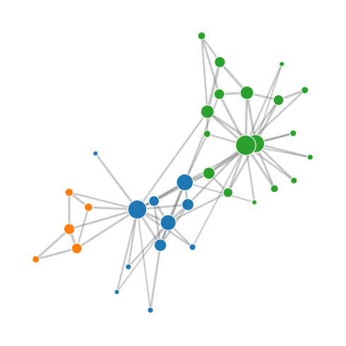
Fig. 7 The example network coloured by the modules read off the result. The same assignment feeds the DataFrame and the per-node iteration above; marker area scales with each node’s flow.

The layout respects the network’s edge structure: tightly connected nodes appear close together, and the colour boundaries show where the random walk crosses between modules.

Comparing trials and inspecting degeneracy

Infomap runs num_trials independent searches and keeps only the best partition. To inspect how consistent the result is, run several single-trial searches from different seeds and compare their codelengths:

codelengths = [
    infomap.run(g, two_level=True, seed=seed, num_trials=1).codelength
    for seed in range(1, 11)
]

print("Codelengths across 10 single-trial runs:")
print(f"  min:    {min(codelengths):.6f}")
print(f"  max:    {max(codelengths):.6f}")
print(f"  range:  {max(codelengths) - min(codelengths):.6f}")
print(f"Best (10-trial run): {result.codelength:.6f}")

Codelengths across 10 single-trial runs:
  min:    4.087423
  max:    4.087423
  range:  0.000000
Best (10-trial run): 4.087423

A tight spread means most trials recover the same strong community structure. A wide spread, or a best-of-10 value below the single-trial minimum, signals a degenerate solution landscape that warrants more trials. The karate club’s community structure is pronounced enough that every trial finds the same codelength; large noisy networks spread wider.

Collecting a sweep into a table

Sweeps over parameters or networks are the common case: vary a knob, keep the per-run metrics. summary() returns those scalars as a plain dict whose keys match the Result property names, so each run drops straight into a one-row-per-run pandas.DataFrame. Add your own swept-parameter columns alongside:

records = []
for markov_time in (0.75, 1.0, 1.5):
    r = infomap.run(g, markov_time=markov_time, seed=123, num_trials=10)
    records.append({"markov_time": markov_time, **r.summary()})

sweep = pd.DataFrame(records)
sweep[["markov_time", "codelength", "num_top_modules", "num_levels"]]

	markov_time	codelength	num_top_modules	num_levels
0	0.75	3.870095	6	2
1	1.00	4.087423	3	2
2	1.50	4.381199	3	2

The same shape covers a sweep over several networks (add a network column). It also covers repeated seeds: add a seed column, then sweep.groupby("markov_time").agg(...) reduces trials to a mean and spread. to_series() is the pandas-native single row, so pandas.DataFrame([r.to_series() for r in results]) builds the same table. Both read only the eagerly captured scalars, so — unlike to_dataframe() — they never go stale after a re-run.

Pitfalls

• A Result goes stale if its network runs again. Reading nodes() or modules() on a Result after a later run() on the same network raises; finish reading a result before you re-run. The eagerly captured scalar properties stay readable.

• Module ids carry no order or meaning. They are stable within one run but arbitrary across runs; compare partitions with a metric, not id equality.

• modules() returns the top level by default. Pass level=-1 for the finest level of a multilevel result.

API pointers

All on Result: metrics codelength, one_level_codelength, relative_codelength_savings, num_top_modules, num_levels; partition accessors modules(), nodes(), to_dataframe(); and the per-run scalar row summary() / to_series().

Going deeper

• API reference is the complete property and method reference for infomap.Result.

• options=Options(converge=True) treats num_trials as a cap and stops once the best codelength plateaus; pair it with a high cap on networks whose degeneracy you have not yet characterised. The solution-landscape tooling follows the solution-landscape clustering approach [Calatayud et al., 2019].

• The survey (§4) covers the multilevel map equation and hierarchical community detection in full [Smiljanić et al., 2026].