Infomap options guide
Infomap has many options. This guide explains what they are for and shows the ones you change most often, grouped by what you want to achieve. For a first end-to-end run, start with the quickstart.
Infomap finds communities by minimizing the map equation, the description length of a random walk on the network [Rosvall et al., 2009, Rosvall and Bergstrom, 2008]. Most options below change how that random walk is defined, how hard the search works, or what gets written. Each section names the paper that introduced the option, and the References section at the end collects them.
Every option is the same idea across interfaces. A command-line flag like
--two-level is the keyword two_level=True in Python and the matching argument
in R. In Python you can set options three ways:
the common keyword arguments
seed,num_trials,two_level,directed, andmarkov_time— these stay oninfomap.run(...)/Infomap(...)a reusable
Optionsobject passed asoptions=toinfomap.run(...)— the home for every other (advanced) option; passing those as bare keyword arguments is pending-deprecated and leaves the signature in 3.0a raw flag string:
Infomap(args="--two-level --num-trials 20")
This guide passes advanced options through the options= carrier. The last section lists every option with its
flag, default, and description, generated from the installed package so it always
matches your version.
import infomap
from infomap import Infomap
import networkx as nx
import pandas as pd
import matplotlib.pyplot as plt
from pathlib import Path
Reproducible runs
Set a seed and a meaningful num_trials so results are reproducible and stable.
This guide fixes seed=123 and num_trials=20. The Python API is quiet by
default; call infomap.enable_log() to see the engine log.
print("Infomap version:", infomap.__version__)

SEED = 123
NUM_TRIALS = 20
Infomap version: 2.15.0
Which option should I change?
Start from your goal and reach for the matching option. Each option has its own section below, and the full reference is at the end.
Your goal |
Options to reach for |
|---|---|
Make results reproducible |
|
Get a better, more stable partition |
|
Get fewer, larger modules |
|
Get more, finer modules |
|
Control the hierarchy depth |
|
Respect link direction |
|
Run faster on large networks |
|
Handle sparse, noisy, or incomplete data |
|
Cluster multilayer or temporal networks |
|
Bias the partition with node metadata |
|
Start from, or only score, a partition |
|
Choose what gets written |
|
For run time and memory planning, see benchmark-performance.
Accuracy: reproducibility and solution quality
Infomap is a stochastic search. A single trial can land in a worse local minimum, so the result depends on the seed. Two options control this.
seedfixes the random number generator so a run is reproducible.num_trialsruns that many independent searches and keeps the best (lowest codelength) one. More trials give a better and more stable result at a higher run time.
Calatayud et al. [2019] found that stochastic searches produce many near-degenerate solutions, so exploring more of the landscape gives a more reliable partition.
def run_jazz(**options):
    return infomap.run("data/jazz.net", options=options)


# A single trial varies with the seed: different seeds find different codelengths.
single_trial = pd.DataFrame(
    {"seed": s, "codelength": round(run_jazz(seed=s, num_trials=1).codelength, 4)}
    for s in range(1, 6)
)
single_trial
| seed | codelength | |
|---|---|---|
| 0 | 1 | 6.9099 |
| 1 | 2 | 6.8647 |
| 2 | 3 | 6.9101 |
| 3 | 4 | 6.8656 |
| 4 | 5 | 6.8650 |
# Keeping the best of many trials gives a lower, stable codelength.
pd.DataFrame(
    {
        "num_trials": nt,
        "codelength": round(run_jazz(seed=SEED, num_trials=nt).codelength, 4),
    }
    for nt in (1, 5, 20, 50)
)
| num_trials | codelength | |
|---|---|---|
| 0 | 1 | 6.9099 |
| 1 | 5 | 6.8647 |
| 2 | 20 | 6.8615 |
| 3 | 50 | 6.8612 |
converge treats the trial count as a cap. It runs trials until the best
codelength stops improving, so you can ask for many trials without always paying
for all of them.
result = run_jazz(seed=SEED, num_trials=50, converge=True)
round(result.codelength, 4)
6.8615
Algorithm: resolution and hierarchy
These options change what partition Infomap looks for, not how hard it searches.
We use two small example networks: networkx’s built-in ring of cliques, and a synthetic nested hierarchy built inline (networkx has no deep-hierarchy generator). The inline helper is notebook-local and is not a public Infomap API.
def hierarchical_graph():
    # Nested structure at three scales: 2 top groups, each with 2 subgroups,
    # each with 2 cliques of 5 nodes. Edge weights shrink with each scale, so the
    # best map is a deep, four-level hierarchy.
    G = nx.Graph()
    nid = 0
    top_groups = []
    for _ in range(2):
        subgroups = []
        for _ in range(2):
            cliques = []
            for _ in range(2):
                members = list(range(nid, nid + 5))
                nid += 5
                for i in range(len(members)):
                    for j in range(i + 1, len(members)):
                        G.add_edge(members[i], members[j], weight=100.0)
                cliques.append(members)
            for a in range(len(cliques)):
                for b in range(a + 1, len(cliques)):
                    G.add_edge(
                        cliques[a][0], cliques[b][0], weight=10.0
                    )  # within subgroup
            subgroups.append(cliques)
        for a in range(len(subgroups)):
            for b in range(a + 1, len(subgroups)):
                G.add_edge(
                    subgroups[a][0][0], subgroups[b][0][0], weight=1.0
                )  # within top group
        top_groups.append(subgroups)
    for a in range(len(top_groups)):
        for b in range(a + 1, len(top_groups)):
            G.add_edge(
                top_groups[a][0][0][0], top_groups[b][0][0][0], weight=0.1
            )  # across top groups
    return G


def run_graph(G, **options):
    return infomap.run(G, seed=SEED, num_trials=NUM_TRIALS, options=options)


G_hier = hierarchical_graph()
G_ring = nx.ring_of_cliques(16, 5)  # networkx built-in: 16 cliques of 5 nodes
two_level versus the default multilevel search
By default Infomap finds a hierarchy with as many levels as the flow supports.
two_level=True forces a single flat level of modules. On the nested
network, the multilevel solution builds a four-level hierarchy under the two top
groups, while the two-level solution reports the eight cliques as one flat level.
Rosvall and Bergstrom [2011] introduced the multilevel map equation, which finds
this depth on its own.
rows = []
for two_level in (False, True):
    result = run_graph(G_hier, two_level=two_level)
    rows.append(
        {
            "two_level": two_level,
            "levels": result.num_levels,
            "top_modules": result.num_top_modules,
            "codelength": round(result.codelength, 4),
        }
    )
pd.DataFrame(rows)
| two_level | levels | top_modules | codelength | |
|---|---|---|---|---|
| 0 | False | 4 | 2 | 2.3762 |
| 1 | True | 2 | 8 | 2.3848 |
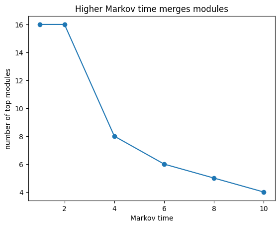
markov_time sets the resolution
markov_time scales how costly it is to move between modules. Higher values make
module boundaries more expensive to cross, so modules merge and you get fewer,
larger ones. Lower values give more, finer modules. It is the main resolution knob.
Kheirkhahzadeh et al. [2016] made sweeping Markov time across scales
efficient.
variable_markov_time instead sets a local time per node, so one run handles
sparse and dense regions at once (Edler et al., 2022).
markov_sweep = pd.DataFrame(
    {
        "markov_time": mt,
        "top_modules": run_graph(
            G_ring, two_level=True, markov_time=mt
        ).num_top_modules,
    }
    for mt in (1, 2, 4, 6, 8, 10)
)
markov_sweep
| markov_time | top_modules | |
|---|---|---|
| 0 | 1 | 16 |
| 1 | 2 | 16 |
| 2 | 4 | 8 |
| 3 | 6 | 6 |
| 4 | 8 | 5 |
| 5 | 10 | 4 |
ax = markov_sweep.plot(x="markov_time", y="top_modules", marker="o", legend=False)
ax.set(
    xlabel="Markov time",
    ylabel="number of top modules",
    title="Higher Markov time merges modules",
)
plt.show()
Steering the module and level counts
When you have a target structure in mind, two soft preferences nudge the search without hard-coding the answer.
preferred_number_of_modulespenalizes solutions whose module count is far from the value you give.preferred_number_of_levelsbiases the hierarchy depth. Steering to a shallower hierarchy is reliable; deeper is best-effort. Usepreferred_number_of_levels_strengthto scale how hard it steers.
pd.DataFrame(
    {
        "preferred_number_of_modules": p,
        "top_modules": run_graph(
            G_ring, two_level=True, preferred_number_of_modules=p
        ).num_top_modules,
    }
    for p in (2, 4, 8, 16)
)
| preferred_number_of_modules | top_modules | |
|---|---|---|
| 0 | 2 | 2 |
| 1 | 4 | 4 |
| 2 | 8 | 8 |
| 3 | 16 | 16 |
rows = []
for levels in (None, 3):
    options = {} if levels is None else {"preferred_number_of_levels": levels}
    result = run_graph(G_hier, **options)
    rows.append(
        {
            "preferred_number_of_levels": levels or "default",
            "levels": result.num_levels,
            "top_modules": result.num_top_modules,
        }
    )
pd.DataFrame(rows)
| preferred_number_of_levels | levels | top_modules | |
|---|---|---|---|
| 0 | default | 4 | 2 |
| 1 | 3 | 3 | 4 |
Flow model: how flow is derived from links
Infomap clusters the flow of a random walker, so the flow model matters. The most common choice is direction.
directed=Truetreats links as directed. It is shorthand forflow_model="directed".flow_modelselects amongundirected,directed,undirdir,outdirdir,rawdir, andprecomputedfor finer control.teleportation_probabilityandrecorded_teleportationadjust how a directed walker teleports and whether those steps are encoded.
On a directed network, respecting direction can change the partition. Lambiotte and Rosvall [2012] introduced smart teleportation, which makes directed results robust to the teleportation rate.
directed_net = nx.DiGraph()
directed_net.add_edges_from([(1, 2), (2, 3), (3, 1), (3, 4), (4, 5), (5, 6), (6, 4)])

rows = []
for flow_model in ("undirected", "directed"):
    result = infomap.run(
        directed_net,
        options=infomap.Options(flow_model=flow_model),
        seed=SEED,
        num_trials=NUM_TRIALS,
    )
    rows.append(
        {
            "flow_model": flow_model,
            "top_modules": result.num_top_modules,
            "codelength": round(result.codelength, 4),
        }
    )
pd.DataFrame(rows)
| flow_model | top_modules | codelength | |
|---|---|---|---|
| 0 | undirected | 2 | 2.3207 |
| 1 | directed | 2 | 1.7731 |
Regularization for sparse, noisy, or incomplete data
Sparse or under-sampled networks can be over-partitioned: Infomap splits on sampling noise instead of real structure. Two options make the partition more conservative.
regularizedadds a fully connected Bayesian prior network, which reduces overfitting to missing links and merges weakly supported modules. Scale it withregularization_strength; larger values merge more.entropy_correctedcorrects the negative entropy bias in small samples, which matters most for solutions with many modules.
Smiljanić et al. [2020] derived both from the Bayesian map equation, which Smiljanić et al. [2021] extended to weighted and directed data.
On the jazz network, regularization steadily merges the least supported modules. When the network has missing links, see Networks with incomplete data for the full treatment.
rows = []
for label, options in [
    ("baseline", {}),
    ("regularized", {"regularized": True}),
    ("regularized, strength 2", {"regularized": True, "regularization_strength": 2.0}),
]:
    result = run_jazz(seed=SEED, num_trials=NUM_TRIALS, **options)
    rows.append(
        {
            "setting": label,
            "top_modules": result.num_top_modules,
            "codelength": round(result.codelength, 4),
        }
    )
pd.DataFrame(rows)
| setting | top_modules | codelength | |
|---|---|---|---|
| 0 | baseline | 6 | 6.8615 |
| 1 | regularized | 5 | 7.2532 |
| 2 | regularized, strength 2 | 4 | 7.4569 |
Multilayer and temporal networks
For multilayer or temporal data, a state node can relax to neighboring layers while the walker moves. These options control that coupling.
multilayer_relax_rateis the probability of relaxing to other layers instead of staying in the current one.multilayer_relax_limit,..._up, and..._downrestrict relaxation to nearby layers, which is useful for ordered (temporal) layers.multilayer_relax_to_selfcouples a state node to its own physical node in the target layer, building a smaller state network with the same flow.
De Domenico et al. [2015] introduced the relax rate in the multiplex map
equation. Edler et al. [2017] cast memory and multilayer networks as one
state-node formulation, and multilayer_relax_by_jsd couples layers by flow
similarity for intermittent communities [Aslak et al., 2018].
Build multilayer input with add_multilayer_intra_link (within a layer) and
add_multilayer_inter_link (between layers), then set the relax options as usual.
ml = infomap.Network()
intra = [(1, 2), (2, 3), (3, 1), (4, 5), (5, 6), (6, 4)]  # two triangles per layer
for layer in (1, 2):
    for source, target in intra:
        ml.add_multilayer_intra_link(layer, source, target, 1.0)
result = ml.run(options=infomap.Options(seed=SEED, num_trials=NUM_TRIALS, multilayer_relax_rate=0.25))
result.num_top_modules
2
The dedicated Multilayer Networks notebook goes further.
Metadata
meta_data reads a node attribute from a clu-format file and encodes it alongside
the network, biasing modules toward the metadata groups. meta_data_rate sets how
strongly the metadata is weighted. Emmons and Mucha [2019] introduced this tunable attribute weight, and
Bassolas et al. [2022] extended it to nonlocal metadata relationships. See
Networks with Metadata
for the theory.
karate = nx.karate_club_graph()

# Write a clu-format metadata file: node id (1-based) and a group id.
Path("output").mkdir(exist_ok=True)
with open("output/karate-club.meta", "w") as f:
    f.write("# node_id metadata\n")
    for node in karate.nodes():
        group = 0 if karate.nodes[node]["club"] == "Mr. Hi" else 1
        f.write(f"{node + 1} {group}\n")

rows = []
for label, options in [
    ("no metadata", {}),
    ("with metadata", {"meta_data": "output/karate-club.meta"}),
]:
    result = run_graph(karate, **options)
    rows.append(
        {
            "setting": label,
            "top_modules": result.num_top_modules,
            "codelength": round(result.codelength, 4),
        }
    )
pd.DataFrame(rows)
| setting | top_modules | codelength | |
|---|---|---|---|
| 0 | no metadata | 3 | 4.0874 |
| 1 | with metadata | 6 | 4.6413 |
Shaping the input
A few options change which network Infomap sees, or reuse an existing partition.
cluster_datareads an initial partition (a.clufile) or a hierarchy (a.tree/.ftreefile) to start from.no_infomapskips the search entirely. Combined withcluster_data, it scores an existing partition without searching, which lets you compare partitions on the same codelength scale.weight_thresholdignores links below a weight, andnode_limitreads only up to a node id. Both trim the input before clustering.
Here we cluster a network, save the partition, then score that same partition without re-running the search.
im = Infomap(seed=SEED, num_trials=NUM_TRIALS)
im.read_file("data/jazz.net")
result = im.run()
result.write_clu("output/jazz.clu")
optimized = round(result.codelength, 4)

scored = infomap.run(
    "data/jazz.net",
    options=infomap.Options(cluster_data="output/jazz.clu", no_infomap=True),
)

pd.DataFrame(
    [
        {"run": "optimized", "codelength": optimized},
        {"run": "scored only (no_infomap)", "codelength": round(scored.codelength, 4)},
    ]
)
| run | codelength | |
|---|---|---|
| 0 | optimized | 6.8615 |
| 1 | scored only (no_infomap) | 6.8615 |
Choosing the output
infomap.run() and Infomap.run() return their results in memory — on the
Python library surface they do not write files by default. Write the native
files straight off the Result:
result.write_tree(path)writes the.treehierarchy,result.write_flow_tree(path)the.ftreevariant (with aggregated links between modules, used by the Network Navigator), andresult.write_clu(path, depth_level=...)the top-level (or chosen-depth).cluassignment.Network.write_pajek(path)/Network.write_state_network(path)serialize the input network itself.
The option flags tree, ftree, clu, output, out_name, and
no_file_output are CLI-only: on the Python library surface they are inert (they
act only through the raw args escape hatch together with an output directory),
so setting them via Options writes nothing and emits a UserWarning. Console
output is controlled by logging — call infomap.enable_log() to see the engine
log.
In a notebook you usually read metrics and node assignments from the Result
object that run returns, for example its to_dataframe(...), and write files
only when another tool needs them.
result = run_graph(karate)

# Read results in memory, no files needed.
result.to_dataframe(columns=["node_id", "module_id", "flow"]).head()
| node_id | module_id | flow | |
|---|---|---|---|
| 0 | 0 | 1 | 0.090909 |
| 1 | 1 | 1 | 0.062771 |
| 2 | 2 | 1 | 0.071429 |
| 3 | 3 | 1 | 0.038961 |
| 4 | 7 | 1 | 0.028139 |
# Or write explicit formats for downstream tools, straight off the Result.
result = infomap.run(karate, seed=SEED, num_trials=NUM_TRIALS)
result.write_clu("output/karate.clu")
result.write_tree("output/karate.tree")
result.write_flow_tree("output/karate.ftree")
sorted(p.name for p in Path("output").glob("karate.*"))
['karate.clu', 'karate.ftree', 'karate.tree']
Full options reference
This guide covers the options you reach for most often. For the complete list, with every flag, default, and description, use any of these:
from infomap import Options
help(Options)
From the command line, infomap --help lists the common options, infomap -hh
adds the advanced ones, and infomap --print-json-parameters prints the full
machine-readable catalog. The API options reference renders
the same Options fields as a searchable web page.
References
The options in this guide come from the map equation literature. The survey [Smiljanić et al., 2026] ties them together; the papers below introduced each one.
Foundations
Rosvall and Bergstrom (2008). Maps of random walks on complex networks reveal community structure. PNAS 105, 1118. https://doi.org/10.1073/pnas.0706851105
Rosvall, Axelsson, and Bergstrom (2009). The map equation. Eur. Phys. J. Special Topics 178, 13. https://doi.org/10.1140/epjst/e2010-01179-1
Smiljanić, Blöcker, Holmgren, Edler, Neuman, and Rosvall (2026). Community Detection with the Map Equation and Infomap: Theory and Applications. ACM Computing Surveys 58(7). https://doi.org/10.1145/3779648
Hierarchy and resolution (two_level, preferred_number_of_levels,
markov_time, variable_markov_time)
Rosvall and Bergstrom (2011). Multilevel compression of random walks on networks reveals hierarchical organization. PLoS ONE 6(4), e18209. https://doi.org/10.1371/journal.pone.0018209
Kawamoto and Rosvall (2015). Estimating the resolution limit of the map equation in community detection. Phys. Rev. E 91, 012809. https://doi.org/10.1103/PhysRevE.91.012809
Kheirkhahzadeh, Lancichinetti, and Rosvall (2016). Efficient community detection of network flows for varying Markov times. Phys. Rev. E 93, 032309. https://doi.org/10.1103/PhysRevE.93.032309
Edler, Smiljanić, Holmgren, Antonelli, and Rosvall (2022). Variable Markov dynamics as a multi-focal lens to map multi-scale complex networks. https://arxiv.org/abs/2211.04287
Flow model and teleportation (flow_model, directed,
teleportation_probability, recorded_teleportation)
Lambiotte and Rosvall (2012). Ranking and clustering of nodes in networks with smart teleportation. Phys. Rev. E 85, 056107. https://doi.org/10.1103/PhysRevE.85.056107
Reliability and regularization (num_trials, converge, regularized,
entropy_corrected)
Calatayud, Bernardo-Madrid, Neuman, Rojas, and Rosvall (2019). Exploring the solution landscape enables more reliable network community detection. Phys. Rev. E 100, 052308. https://doi.org/10.1103/PhysRevE.100.052308
Smiljanić, Edler, and Rosvall (2020). Mapping flows on sparse networks with missing links. Phys. Rev. E 102, 012302. https://doi.org/10.1103/PhysRevE.102.012302
Smiljanić, Blöcker, Edler, and Rosvall (2021). Mapping flows on weighted and directed networks with incomplete observations. J. Complex Netw. 9, cnab044. https://doi.org/10.1093/comnet/cnab044
Higher-order, multilayer, metadata, and bipartite (multilayer_relax_*,
meta_data, bipartite options)
Rosvall, Esquivel, Lancichinetti, West, and Lambiotte (2014). Memory in network flows and its effects on spreading dynamics and community detection. Nature Commun. 5, 4630. https://doi.org/10.1038/ncomms5630
De Domenico, Lancichinetti, Arenas, and Rosvall (2015). Identifying modular flows on multilayer networks reveals highly overlapping organization. Phys. Rev. X 5, 011027. https://doi.org/10.1103/PhysRevX.5.011027
Edler, Bohlin, and Rosvall (2017). Mapping higher-order network flows in memory and multilayer networks with Infomap. Algorithms 10, 112. https://doi.org/10.3390/a10040112
Aslak, Rosvall, and Lehmann (2018). Constrained information flows in temporal networks reveal intermittent communities. Phys. Rev. E 97, 062312. https://doi.org/10.1103/PhysRevE.97.062312
Emmons and Mucha (2019). Map equation with metadata: varying the role of attributes in community detection. Phys. Rev. E 100, 022301. https://doi.org/10.1103/PhysRevE.100.022301
Blöcker and Rosvall (2020). Mapping flows on bipartite networks. Phys. Rev. E 102, 052305. https://doi.org/10.1103/PhysRevE.102.052305
Bassolas, Holmgren, Marot, Rosvall, and Nicosia (2022). Mapping nonlocal relationships between metadata and network structure. Sci. Adv. 8, eabn7558. https://doi.org/10.1126/sciadv.abn7558
How to cite
If you use Infomap in published work, mapequation.org recommends citing two things: the map equation paper [Rosvall and Bergstrom, 2008] for the method, and the MapEquation software package [Edler et al., 2026] for the implementation and version. See How to cite for BibTeX.
Where to go next
quickstart for a first end-to-end run.
benchmark-performance to plan run time and memory for the accuracy and speed options.
The Infomap user guide documents file formats and the algorithm in depth.