Hierarchy and the multilevel map equation¶
Concept
At a glance
The multilevel map equation lets Infomap discover how many levels of nested structure your network contains, with no resolution parameter to tune.
Limits of a two-level partition¶
Real networks rarely organise into one flat layer of modules. Scientific disciplines hold sub-fields that hold research topics, and cities hold neighbourhoods that hold blocks. A plain two-level partition, one index codebook over one set of leaf modules, sees only one cross-section of that structure at a time.
The two-level map equation has a resolution limit [Kawamoto and Rosvall, 2015]: modules with too few internal links go missing, because merging them into a larger module shortens the two-level description. The threshold grows with the logarithm of the total boundary-crossing traffic; the toggle below gives the exact bound. In a nested network the two-level method must choose between resolving the fine-grained modules and capturing the coarse super-groups.
The multilevel map equation lifts the limit by allowing nested index codebooks
to any depth. It adds a level only when that level shortens the total
description, so the depth of the output tree is read off the data. Multilevel is
the default; pass two_level=True to disable it.
Nested addresses¶
Think of the two-level map as a street address with two parts: city and street. That works for a small country. For the whole world you need at least country → city → street, and for a large nation country → state → city → street. Each extra level earns its place only when travellers stay inside the smaller unit often enough that the added name pays for itself in shorter directions overall.
The multilevel map equation applies the same logic to random-walk descriptions. Each level of hierarchy adds a set of nested codebooks. When a walker stays inside a module for a long time, giving that module its own sub-codebook for the nodes it visits shortens the description. The same objective, description length, decides whether to add another sub-level: Infomap keeps adding levels until none shortens the description, then stops.
The result is a tree of modules. Each leaf is a network node. Internal tree nodes are modules at different granularities. You can read off the coarse super-group membership at depth 1, the fine-grained triangle membership at depth 2, and so on.
Nested codebooks¶
The two-level map equation (see the map equation chapter) uses one index codebook to describe inter-module movements and one codebook per module to describe intra-module node visits:
The hierarchical extension [Rosvall and Bergstrom, 2011] replaces the single index codebook with a tree of nested index codebooks. Each module \(i\) at the top level has its own sub-index codebook \(\mathcal{Q}^i\) for directing the random walker among its sub-modules, and those sub-modules may have their own sub-sub-index codebooks, and so on. The total description length becomes a recursive sum:
where each sub-map \(\mathsf{M}^i\) contributes
and the recursion bottoms out at the leaf level with
The rate \(q_{\circlearrowright}^i\) at which the walker uses module \(i\)’s sub-index codebook depends on the local traffic within module \(i\), not on a global cut size that grows with the whole network. This is why the resolution limit relaxes; see [Kawamoto and Rosvall, 2015], §IV.
Infomap searches for the hierarchical partition that minimises the total \(L\) using a fast stochastic recursive algorithm: it first generates top-level modules, then recursively applies the same procedure inside each module to find sub-modules, adding or removing levels wherever the description shortens. The search converges to a locally optimal hierarchical tree.
Resolution limit: why two-level fails and hierarchy helps
The two-level map equation’s resolution limit can be derived analytically [Kawamoto and Rosvall, 2015]. For an undirected network with cut size \(C\) (total number of links crossing module boundaries), the two-level method can fail to detect a module with \(l_c\) internal links when
Contrast this with modularity, whose resolution limit grows with the size of the whole network: it cannot resolve communities with fewer than roughly \(\sqrt{m/2}\) internal links, where \(m\) is the total link count (see Reading Infomap through Louvain and Leiden). The map equation’s dependence on the local cut size \(C\) rather than the global \(m\) is already much less restrictive, but it does not vanish.
The hierarchical map equation evaluates the analogous update with the effective network size equal to the super-module plus its boundary links, not the full graph. Because a super-module is much smaller than the full network, the cut size that gates a fine-level split is tiny, so the search resolves fine-level modules that the two-level stage would swallow. For networks with a pronounced nested structure the hierarchical method all but eliminates the resolution limit; see [Kawamoto and Rosvall, 2015], §IV.
Nine triangles, three super-groups¶
The nine-triangles network from the examples on mapequation.org is built for
exactly this: twenty-seven nodes in nine triangles, arranged in three
super-groups of three triangles each. Weight-1 links join the triangles inside
a super-group; the three links between super-groups are weaker, 0.8. We build
it by hand and let Infomap find the nesting automatically; it also ships
ready-made as infomap.datasets.nine_triangles().
Build the network¶
import networkx as nx
import infomap

links = []

# Nine triangles: nodes {1, 2, 3}, {4, 5, 6}, ..., {25, 26, 27}
for t in range(9):
    a, b, c = 3 * t + 1, 3 * t + 2, 3 * t + 3
    links += [(a, b, 1.0), (a, c, 1.0), (b, c, 1.0)]

# Weight-1 links join the three triangles inside each super-group
for base in (0, 9, 18):
    links += [
        (base + 2, base + 4, 1.0),
        (base + 3, base + 7, 1.0),
        (base + 6, base + 8, 1.0),
    ]

# Weaker links join the three super-groups into a ring
links += [(5, 10, 0.8), (9, 19, 0.8), (18, 23, 0.8)]

G = nx.Graph()
for u, v, w in links:
    G.add_edge(u, v, weight=w)

print(f"Nodes: {G.number_of_nodes()}, Edges: {G.number_of_edges()}")
Nodes: 27, Edges: 39
Run multilevel Infomap¶
from infomap import Network, run

net = Network()
for u, v, w in links:
    net.add_link(u, v, w)
result = run(net, num_trials=10, seed=123)

print(f"Tree depth (num_levels): {result.num_levels}")
print(f"Top-level modules:       {result.num_top_modules}")
print(f"Map equation codelength: {result.codelength:.4f} bits/step")

# The text below reads these exact counts; assert so the build catches drift.
assert result.num_top_modules == 3

# The bundled copy is the same network; the two must agree exactly.
result_pkg = infomap.run(infomap.datasets.nine_triangles(),
                         num_trials=10, seed=123)
assert result.codelength == result_pkg.codelength
Tree depth (num_levels): 3
Top-level modules:       3
Map equation codelength: 3.3858 bits/step
As num_levels shows, the tree runs from a root through three coarse
super-groups down to the nine fine triangles.
Read module assignments at each level¶
# Coarsest level (depth 1): the three super-groups
modules_l1 = result.modules(depth=1)

# Finer level (depth 2): the nine individual triangles
modules_l2 = result.modules(depth=2)

print("Level-1 assignment (super-groups):")
print(modules_l1)

print("\nLevel-2 assignment (triangles):")
print(modules_l2)

assert len(set(modules_l2.values())) == 9
Level-1 assignment (super-groups):
{7: 1, 8: 1, 9: 1, 4: 1, 6: 1, 5: 1, 2: 1, 3: 1, 1: 1, 16: 2, 17: 2, 18: 2, 11: 2, 12: 2, 10: 2, 13: 2, 15: 2, 14: 2, 20: 3, 21: 3, 19: 3, 22: 3, 24: 3, 23: 3, 25: 3, 26: 3, 27: 3}

Level-2 assignment (triangles):
{7: 1, 8: 1, 9: 1, 4: 2, 6: 2, 5: 2, 2: 3, 3: 3, 1: 3, 16: 4, 17: 4, 18: 4, 11: 5, 12: 5, 10: 5, 13: 6, 15: 6, 14: 6, 20: 7, 21: 7, 19: 7, 22: 8, 24: 8, 23: 8, 25: 9, 26: 9, 27: 9}
Pass depth=-1 for the finest (leaf) level whatever the tree depth.
Visualise both levels side by side¶
from myst_nb import glue

import matplotlib.pyplot as plt
from docs_viz import draw_partition

fig, axes = plt.subplots(1, 2, figsize=(9, 4), layout="constrained")

# Same flow in both panels; only the level of the grouping differs.
flow = {n.node_id: n.flow for n in result.nodes()}

draw_partition(G, modules_l1, ax=axes[0], flow=flow)
axes[0].set_title("Level 1: super-groups", fontsize=11)

draw_partition(G, modules_l2, ax=axes[1], flow=flow)
axes[1].set_title("Level 2: triangles", fontsize=11)

fig.suptitle("Two levels of hierarchy, discovered automatically", fontsize=12)
glue("fig-hierarchy-and-the-multilevel-map", fig, display=False)
plt.close(fig)
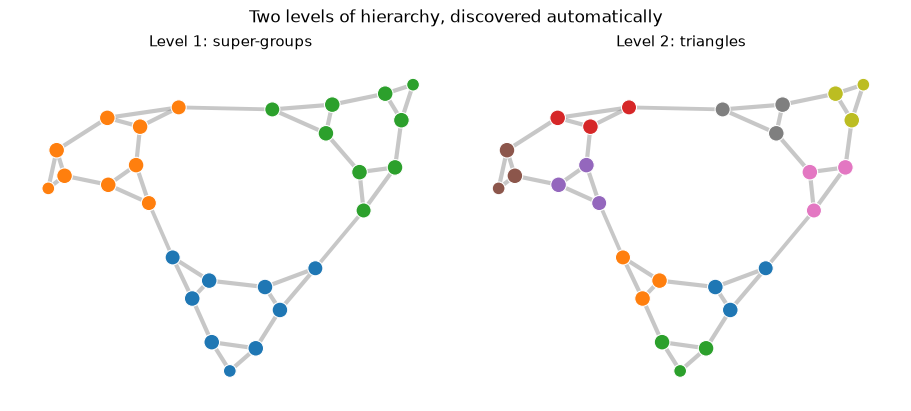
Fig. 3 The same nested network at two levels of the hierarchy Infomap discovers. Left: the three coarse super-groups. Right: the nine fine triangles nested inside them. Both panels share one layout, so the levels read against each other.¶
This matches the theoretical picture [Rosvall and Bergstrom, 2011]: the network has dense intra-triangle flow, moderately dense intra-super-group flow (the unit-weight links joining a super-group’s triangles), and weak inter-super-group flow (the three 0.8 links). Three nested levels of codebooks capture exactly those three scales (two levels of index codebooks over the module codebooks), and the hierarchical map equation confirms that the three-level description is more compressed than either a flat two-level partition or a one-level description.
API pointers¶
All on Result: num_levels (alias
max_depth), num_top_modules,
modules() (pass depth=k, or depth=-1 for the leaf
level), and effective_num_modules(); see
Reading the result. The engine option
two_level=True restricts the search to two levels — leave it off for the full
hierarchy.
Going deeper¶
Source paper for the multilevel map equation [Rosvall and Bergstrom, 2011]; the resolution limit it relaxes is derived in [Kawamoto and Rosvall, 2015].
The survey (§3) adds the multilevel derivation and worked examples [Smiljanić et al., 2026].