Performance and run planning

Estimate an Infomap run’s wall time and peak memory before you start it, and choose threads, trials, and --two-level for your network.

These numbers come from one machine (see How this was measured), so read them as scaling laws you can extrapolate from: time and memory grow with network size, threads, trials, and hierarchy depth in ways that carry across hardware.

What you get

1. How time and memory scale with network size (links), by type.

2. How threads help, and why that depends on hierarchy depth.

3. Why sequential trials cost time but not memory.

4. When --two-level pays off.

5. The cost of hierarchy depth.

6. A table of realistic anchor runs to calibrate against.

7. A recipe for estimating your own run.

By default this page renders measurements committed to data/benchmark-results.csv. To reproduce them, set RUN_BENCHMARK = True in the configuration cell and re-run (about an hour for the full campaign). That overwrites the CSV, and every figure below then reflects your machine.

from pathlib import Path
import pandas as pd
import numpy as np
import matplotlib.pyplot as plt

# --- configuration ---
RUN_BENCHMARK = (
    False  # True regenerates data/benchmark-results.csv on this machine (~1 h)
)
DATA = Path("data/benchmark-results.csv")
SEED = 123
TYPE_COLOR = {"ordinary": "#1f77b4", "state": "#d62728", "multilayer": "#2ca02c"}
plt.rcParams.update({"figure.dpi": 110, "axes.grid": True, "grid.alpha": 0.3})

How this was measured

We measured the committed data on an Apple M2 Pro (8 performance + 4 efficiency cores), 16 GB RAM, macOS, with Infomap 2.12.0 built in release mode with OpenMP (make build-native MODE=release OPENMP=1). The same protocol applies if you re-run:

• We record wall time and peak resident memory for the whole process (/usr/bin/time -l reports real time and maximum resident set size): read, build, optimize, output. That is what you wait for and what has to fit in RAM.

• Each point runs a few times and we report the median, since peak RSS varies by a few hundred MB between runs.

• Every run pins a fixed seed (-s 123) and an explicit thread count (--num-threads N); Infomap otherwise defaults to auto, all cores.

• The synthetic block-model networks hold average degree near 10, so link count is a clean size axis and node count scales with it.

# --- reproduction: reproducible generators + measurement (runs only if RUN_BENCHMARK) ---
# Self-contained campaign that regenerates data/benchmark-results.csv. Networks use
# numpy's legacy RandomState, whose stream is frozen across numpy versions (NEP 19) --
# unlike default_rng, whose Generator methods may change between releases -- so the same
# seed yields byte-identical nets on any machine/numpy and the committed CSV is
# reproducible. macOS-oriented (uses /usr/bin/time -l for peak RSS).
import os
import subprocess
import tempfile


def _find_infomap():
    for c in (Path.cwd(), *Path.cwd().parents):
        if (c / "src" / "main.cpp").exists():
            exe = c / ("Infomap.exe" if os.name == "nt" else "Infomap")
            if not exe.exists():
                raise FileNotFoundError(
                    "Build the CLI first: make build-native MODE=release OPENMP=1"
                )
            return exe
    raise RuntimeError("Run from an Infomap source checkout.")


def _block_targets(rng, src, n, block_size, p_in):
    m = len(src)
    tgt = rng.randint(0, n, size=m, dtype=np.int64)
    in_block = rng.random_sample(m) < p_in
    off = rng.randint(0, block_size, size=int(in_block.sum()), dtype=np.int64)
    tgt[in_block] = np.minimum((src[in_block] // block_size) * block_size + off, n - 1)
    return tgt


def _gen(kind, links, path, seed=SEED, states=2, layers=4, p_in=0.9):
    rng = np.random.RandomState(seed)
    n = max(1, links // 10)
    n_blocks = max(2, n // 200)
    block_size = max(1, n // n_blocks)
    src = rng.randint(0, n, size=links, dtype=np.int64)
    tgt = _block_targets(rng, src, n, block_size, p_in)
    with open(path, "w") as f:
        if kind == "ordinary":
            f.write("*Vertices\n")
            ids = np.arange(n)
            np.savetxt(
                f,
                np.c_[ids, np.char.add(np.char.add('"', ids.astype("U10")), '"')],
                fmt="%s",
            )
            f.write("*Edges\n")
            np.savetxt(f, np.c_[src, tgt], fmt="%d")
        elif (
            kind == "state"
        ):  # `states` memory states per physical node; stateId = phys*states + mem
            f.write("*Vertices\n")
            ids = np.arange(n)
            np.savetxt(
                f,
                np.c_[ids, np.char.add(np.char.add('"', ids.astype("U10")), '"')],
                fmt="%s",
            )
            f.write("*States\n")
            sid = np.concatenate([ids * states + k for k in range(states)])
            phys = np.concatenate([ids for _ in range(states)])
            np.savetxt(f, np.c_[sid, phys], fmt="%d")
            f.write("*Links\n")
            sm = rng.randint(0, states, size=links, dtype=np.int64)
            tm = rng.randint(0, states, size=links, dtype=np.int64)
            np.savetxt(f, np.c_[src * states + sm, tgt * states + tm], fmt="%d")
        else:  # multilayer: inter links (10%) join a node across layers
            layer1 = rng.randint(0, layers, size=links, dtype=np.int64)
            inter = rng.random_sample(links) < 0.1
            layer2 = layer1.copy()
            layer2[inter] = (
                layer1[inter]
                + 1
                + rng.randint(0, layers - 1, size=int(inter.sum()), dtype=np.int64)
            ) % layers
            tgt[inter] = src[inter]
            f.write("*Multilayer\n")
            np.savetxt(f, np.c_[layer1, src, layer2, tgt], fmt="%d")
    return path


def _gen_depth(path, branching, leaf=50, lpn=10, decay=0.15, seed=SEED):
    rng = np.random.RandomState(seed)
    k = len(branching)
    nleaf = int(np.prod(branching))
    n = nleaf * leaf
    m = n * lpn
    src = np.repeat(np.arange(n, dtype=np.int64), lpn)
    leafid = src // leaf
    digits = np.zeros((m, k), dtype=np.int64)
    rem = leafid.copy()
    for j in range(k - 1, -1, -1):
        digits[:, j] = rem % branching[j]
        rem //= branching[j]
    pd_ = (decay ** (k - np.arange(k + 1))).astype(float)
    pd_ /= pd_.sum()
    d = rng.choice(k + 1, size=m, p=pd_)
    tdig = digits.copy()
    for j in range(k):
        msk = j >= d
        c = int(msk.sum())
        if c:
            tdig[msk, j] = rng.randint(0, branching[j], size=c, dtype=np.int64)
    tleaf = np.zeros(m, dtype=np.int64)
    for j in range(k):
        tleaf = tleaf * branching[j] + tdig[:, j]
    tgt = tleaf * leaf + rng.randint(0, leaf, size=m, dtype=np.int64)
    w = decay ** (k - d)
    keep = src != tgt
    with open(path, "w") as f:
        f.write("*Edges\n")
        np.savetxt(f, np.c_[src[keep], tgt[keep], w[keep]], fmt=["%d", "%d", "%.4g"])
    return path


def _measure(
    exe, net, threads, trials, two_level, reps, links, nodes, block, label, typ
):
    rows = []
    for r in range(1, reps + 1):
        with tempfile.TemporaryDirectory() as out:
            cmd = [
                "/usr/bin/time",
                "-l",
                str(exe),
                str(net),
                out,
                "--num-threads",
                str(threads),
                "-N",
                str(trials),
                "-s",
                str(SEED),
            ]
            if two_level:
                cmd.append("-2")
            p = subprocess.run(cmd, capture_output=True, text=True)
        if p.returncode != 0:
            raise RuntimeError(
                f"Infomap failed (exit {p.returncode}) for {label!r}:\n{p.stderr[-800:]}"
            )
        err = p.stderr
        wall = next(
            (
                float(p2[p2.index("real") - 1])
                for t in err.splitlines()
                for p2 in (t.split(),)
                if "real" in p2
            ),
            None,
        )
        rss = next(
            (
                round(float(t.split()[0]) / 1048576, 1)
                for t in err.splitlines()
                if "maximum resident set size" in t
            ),
            None,
        )
        lvl = next(
            (
                int(t.split()[1])
                for t in p.stdout.splitlines()
                if t.strip().startswith("Levels")
            ),
            None,
        )
        cl = next(
            (
                float(t.split()[-1])
                for t in p.stdout.splitlines()
                if "Best codelength" in t
            ),
            None,
        )
        rows.append(
            dict(
                block=block,
                label=label,
                type=typ,
                links=links,
                nodes=nodes,
                threads=threads,
                trials=trials,
                flags="-2" if two_level else "",
                repeat=r,
                wall_s=wall,
                peak_rss_mb=rss,
                levels=lvl,
                codelength=cl,
            )
        )
    return rows


if RUN_BENCHMARK:
    import sys as _sys

    if _sys.platform != "darwin":
        raise RuntimeError(
            "Regeneration uses macOS `/usr/bin/time -l` for peak RSS; "
            "on Linux adapt _measure (e.g. GNU `time -v` or psutil)."
        )
    exe = _find_infomap()
    rows = []
    tmp = Path(tempfile.mkdtemp(prefix="im-guide-"))

    def net(kind, L):
        return _gen(kind, L, tmp / f"{kind}_{L}.net")

    # Block 1: size sweep (8 threads, 1 trial, multilevel)
    for L in [500_000, 1_000_000, 2_000_000, 5_000_000, 10_000_000, 20_000_000]:
        rows += _measure(
            exe,
            net("ordinary", L),
            8,
            1,
            False,
            2 if L >= 10_000_000 else 3,
            L,
            L // 10,
            "B1",
            f"ord_L{L}",
            "ordinary",
        )
    for L in [500_000, 1_000_000, 2_000_000, 5_000_000]:
        rows += _measure(
            exe,
            net("state", L),
            8,
            1,
            False,
            2 if L >= 5_000_000 else 3,
            L,
            L // 10,
            "B1",
            f"state_L{L}",
            "state",
        )
    for L in [1_000_000, 2_000_000, 5_000_000]:
        rows += _measure(
            exe,
            net("multilayer", L),
            8,
            1,
            False,
            2,
            L,
            L // 10,
            "B1",
            f"ml_L{L}",
            "multilayer",
        )
    ord5, st2, ml2 = (
        net("ordinary", 5_000_000),
        net("state", 2_000_000),
        net("multilayer", 2_000_000),
    )
    # Block 2: threads
    for T in [1, 2, 4, 8, 10, 12]:
        rows += _measure(
            exe, ord5, T, 1, False, 3, 5_000_000, 500_000, "B2", f"ord_T{T}", "ordinary"
        )
        rows += _measure(
            exe, st2, T, 1, False, 3, 2_000_000, 200_000, "B2", f"state_T{T}", "state"
        )
    for T in [1, 8]:
        rows += _measure(
            exe, ml2, T, 1, False, 2, 2_000_000, 200_000, "B2", f"ml_T{T}", "multilayer"
        )
    # Block 3: trials (sequential, 8 threads)
    for N in [1, 2, 5, 10]:
        rows += _measure(
            exe,
            ord5,
            8,
            N,
            False,
            2 if N >= 10 else 3,
            5_000_000,
            500_000,
            "B3",
            f"ord_N{N}",
            "ordinary",
        )
        rows += _measure(
            exe,
            st2,
            8,
            N,
            False,
            2 if N >= 10 else 3,
            2_000_000,
            200_000,
            "B3",
            f"state_N{N}",
            "state",
        )
    # Block 4: two-level vs multilevel (flat nets)
    for tl, tag in [(False, "multi"), (True, "2lvl")]:
        rows += _measure(
            exe, ord5, 8, 1, tl, 3, 5_000_000, 500_000, "B4", f"ord_{tag}", "ordinary"
        )
        rows += _measure(
            exe, st2, 8, 1, tl, 3, 2_000_000, 200_000, "B4", f"state_{tag}", "state"
        )
        rows += _measure(
            exe, ml2, 8, 1, tl, 2, 2_000_000, 200_000, "B4", f"ml_{tag}", "multilayer"
        )
    # Block 4b: depth sweep (record real links/nodes from each generated net)
    for nm, br in [
        ("d1", [10000]),
        ("d2", [100, 100]),
        ("d3", [22, 22, 22]),
        ("d4", [10, 10, 10, 10]),
        ("d5", [7, 6, 6, 6, 6]),
    ]:
        dn = _gen_depth(tmp / f"depth_{nm}.net", br)
        dlinks = sum(1 for ln in open(dn) if ln[:1] not in ("*", "#"))
        dnodes = int(np.prod(br)) * 50  # leaf size used by _gen_depth
        rows += _measure(
            exe, dn, 8, 1, False, 3, dlinks, dnodes, "B4b", f"depth_{nm}", "ordinary"
        )
    # Block 2deep / 4deep: threads + two-level on a DEEP net (depth d5, ~6 levels)
    deep = _gen_depth(tmp / "deep.net", [7, 6, 6, 6, 6])
    dl = sum(1 for ln in open(deep) if ln[:1] not in ("*", "#"))
    for T in [1, 2, 4, 8, 10, 12]:
        rows += _measure(
            exe, deep, T, 1, False, 3, dl, 453600, "B2deep", f"deep_T{T}", "ordinary"
        )
    for tl, tag in [(False, "multi"), (True, "2lvl")]:
        rows += _measure(
            exe, deep, 8, 1, tl, 3, dl, 453600, "B4deep", f"deep_{tag}", "ordinary"
        )
    # Block 5: anchors
    A = [
        ("a_ord1M_N1_t1", "ordinary", 1_000_000, 1, 1, 3),
        ("a_ord5M_N10_t10", "ordinary", 5_000_000, 10, 10, 3),
        ("a_ord20M_N10_t10", "ordinary", 20_000_000, 10, 10, 2),
        ("a_state1M_N10_t10", "state", 1_000_000, 10, 10, 3),
        ("a_state5M_N10_t10", "state", 5_000_000, 10, 10, 2),
        ("a_ml2M_N1_t8", "multilayer", 2_000_000, 1, 8, 3),
    ]
    for lab, ty, L, N, T, rp in A:
        rows += _measure(exe, net(ty, L), T, N, False, rp, L, L // 10, "B5", lab, ty)
    pd.DataFrame(rows).to_csv(DATA, index=False)
    print(f"wrote {len(rows)} rows to {DATA}")

# --- load committed (or freshly generated) measurements and reduce to medians ---
raw = pd.read_csv(DATA)
for c in [
    "links",
    "nodes",
    "threads",
    "trials",
    "wall_s",
    "peak_rss_mb",
    "levels",
    "codelength",
]:
    raw[c] = pd.to_numeric(raw[c], errors="coerce")
raw["flags"] = raw["flags"].fillna("")

keys = ["block", "label", "type", "links", "nodes", "threads", "trials", "flags"]
summary = (
    raw.groupby(keys, dropna=False)
    .agg(
        wall_s=("wall_s", "median"),
        peak_rss_mb=("peak_rss_mb", "median"),
        levels=("levels", "max"),
        codelength=("codelength", "median"),
        reps=("repeat", "count"),
    )
    .reset_index()
)
summary["GB"] = summary["peak_rss_mb"] / 1024
summary["Mlinks_per_s"] = summary["links"] / summary["wall_s"] / 1e6
summary["bytes_per_link"] = (
    summary["peak_rss_mb"] * 1048576 / summary["links"].replace(0, np.nan)
)


def blk(b):
    return summary[summary.block == b]


print(f"{len(raw)} raw runs -> {len(summary)} configurations")

166 raw runs -> 60 configurations

1. How time and memory scale with network size

These are your clearest planning levers. With average degree near 10, both grow with the number of links: memory close to linearly, time a little faster (about links^1.2). Network type sets the offset. State (higher-order) networks cost roughly 2× an ordinary one at the same link count, and multilayer costs about 6× the time and 2.4× the memory, because expanding the multilayer input into a state network dominates the work.

b1 = blk("B1")
fig, (ax1, ax2) = plt.subplots(1, 2, figsize=(12, 4.6))
for typ in ["ordinary", "state", "multilayer"]:
    d = b1[b1.type == typ].sort_values("links")
    ax1.plot(d.links, d.wall_s, "o-", color=TYPE_COLOR[typ], label=typ)
    ax2.plot(d.links, d.peak_rss_mb, "o-", color=TYPE_COLOR[typ], label=typ)
for ax, ylab in [(ax1, "wall time (s)"), (ax2, "peak RSS (MB)")]:
    ax.set_xscale("log")
    ax.set_yscale("log")
    ax.set_xlabel("links")
    ax.set_ylabel(ylab)
    ax.legend()
ax1.set_title("Time vs network size (8 threads, 1 trial)")
ax2.set_title("Memory vs network size (8 threads, 1 trial)")
plt.tight_layout()
plt.show()

# Normalized headline metrics — use these to extrapolate to your own network
norm = (
    b1.groupby("type")
    .agg(
        Mlinks_per_s=("Mlinks_per_s", "median"),
        bytes_per_link=("bytes_per_link", "median"),
        lo=("links", "min"),
        hi=("links", "max"),
    )
    .reset_index()
)
norm["links measured"] = norm.apply(
    lambda r: f"{r.lo / 1e6:g}M-{r.hi / 1e6:g}M", axis=1
)
norm = norm[["type", "links measured", "Mlinks_per_s", "bytes_per_link"]]
norm.columns = [
    "type",
    "links measured",
    "throughput (M links/s, 8 threads)",
    "memory (bytes/link)",
]
norm.round(2)

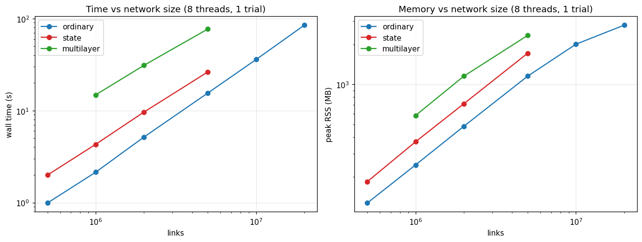
	type	links measured	throughput (M links/s, 8 threads)	memory (bytes/link)
0	multilayer	1M-5M	0.06	604.90
1	ordinary	0.5M-20M	0.35	247.57
2	state	0.5M-5M	0.22	380.79

For one trial on this machine:

• peak memory ≈ links × bytes-per-link (10M-link ordinary ≈ 10M × 250 B ≈ 2.5 GB)

• time ≈ links ÷ throughput (10M-link ordinary ≈ 10M ÷ 0.35M/s ≈ 29 s)

On 16 GB of RAM, memory becomes the binding constraint around 60M links for ordinary networks, 40M for state, and 25M for multilayer.

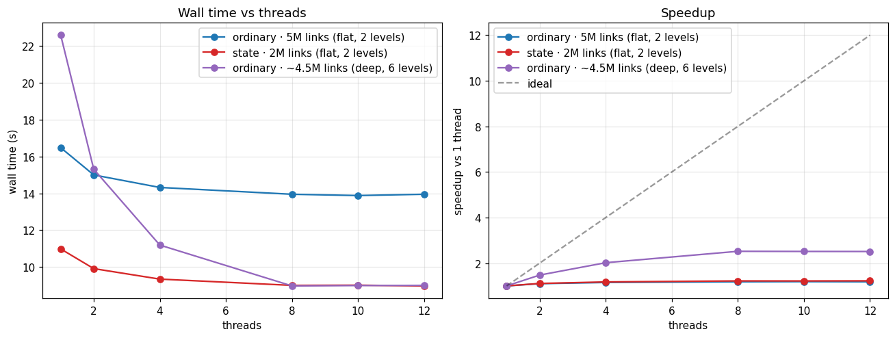
2. Threads: how much they help depends on depth

Infomap parallelizes the recursive, multi-level part of the search; the top-level partition runs serially. How much threads help therefore depends on how deep the hierarchy is.

• A flat (two-level) partition barely moves: about 1.1–1.2× even at 12 threads.

• A deep, hierarchical network reaches about 2.5× and plateaus near 8 threads. The 4 efficiency cores (threads 9–12) contribute little.

Choose the thread count from your network’s structure rather than its size. Past 8 threads you gain little on this hardware.

fig, (ax1, ax2) = plt.subplots(1, 2, figsize=(12, 4.6))
series = [
    ("B2", "ordinary", TYPE_COLOR["ordinary"], "ordinary · 5M links (flat, 2 levels)"),
    ("B2", "state", TYPE_COLOR["state"], "state · 2M links (flat, 2 levels)"),
    ("B2deep", "ordinary", "#9467bd", "ordinary · ~4.5M links (deep, 6 levels)"),
]
for b, typ, color, lab in series:
    d = summary[(summary.block == b) & (summary.type == typ)].sort_values("threads")
    if d.empty:
        continue
    base = d[d.threads == 1].wall_s.iloc[0]
    ax1.plot(d.threads, d.wall_s, "o-", color=color, label=lab)
    ax2.plot(d.threads, base / d.wall_s, "o-", color=color, label=lab)
ax2.plot([1, 12], [1, 12], "k--", alpha=0.4, label="ideal")
ax1.set_xlabel("threads")
ax1.set_ylabel("wall time (s)")
ax1.set_title("Wall time vs threads")
ax1.legend()
ax2.set_xlabel("threads")
ax2.set_ylabel("speedup vs 1 thread")
ax2.set_title("Speedup")
ax2.legend()
plt.tight_layout()
plt.show()

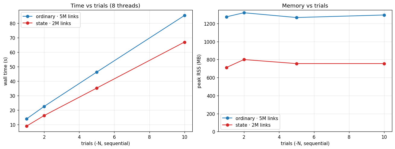
3. Trials cost time, not memory

--num-trials N runs the search N times and keeps the best partition. By default the trials run one after another, so wall time is about (read + build) + N × (one optimization) and peak memory stays flat. More trials raise your chance of hitting the optimum at a predictable, linear time cost and no memory cost.

fig, (ax1, ax2) = plt.subplots(1, 2, figsize=(12, 4.6))
for typ in ["ordinary", "state"]:
    d = blk("B3")[blk("B3").type == typ].sort_values("trials")
    lab = f"{typ} · {d.links.iloc[0] / 1e6:g}M links"
    ax1.plot(d.trials, d.wall_s, "o-", color=TYPE_COLOR[typ], label=lab)
    ax2.plot(d.trials, d.peak_rss_mb, "o-", color=TYPE_COLOR[typ], label=lab)
ax1.set_xlabel("trials (-N, sequential)")
ax1.set_ylabel("wall time (s)")
ax1.set_title("Time vs trials (8 threads)")
ax1.legend()
ax2.set_xlabel("trials (-N, sequential)")
ax2.set_ylabel("peak RSS (MB)")
ax2.set_title("Memory vs trials")
ax2.set_ylim(bottom=0)
ax2.legend()
plt.tight_layout()
plt.show()

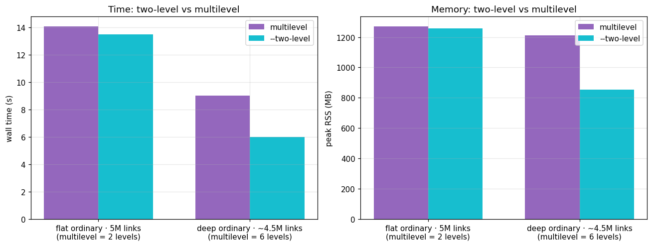
4. --two-level: worth it when the hierarchy is deep

-2 skips the multi-level recursion and returns a flat partition. When the best solution is already shallow, it changes little. On a deep network it runs about 1.5× faster and uses about 30% less memory, because it never builds the hierarchy. Use it when you only need the community level, or when a deep network is pushing your memory limit.

def pair(b, multi, two):
    m = summary[(summary.block == b) & (summary.label == multi)]
    t = summary[(summary.block == b) & (summary.label == two)]
    return (m.iloc[0], t.iloc[0]) if len(m) and len(t) else None


pairs = [
    (
        "flat ordinary · 5M links\n(multilevel = 2 levels)",
        pair("B4", "ord_multi", "ord_2lvl"),
    ),
    (
        "deep ordinary · ~4.5M links\n(multilevel = 6 levels)",
        pair("B4deep", "deep_multi", "deep_2lvl"),
    ),
]
pairs = [(lab, p) for lab, p in pairs if p]
x = np.arange(len(pairs))
bw = 0.36
fig, (axw, axr) = plt.subplots(1, 2, figsize=(12, 4.6))
for ax, attr, ylab, title in [
    (axw, "wall_s", "wall time (s)", "Time: two-level vs multilevel"),
    (axr, "peak_rss_mb", "peak RSS (MB)", "Memory: two-level vs multilevel"),
]:
    ax.bar(
        x - bw / 2,
        [getattr(p[0], attr) for _, p in pairs],
        bw,
        label="multilevel",
        color="#9467bd",
    )
    ax.bar(
        x + bw / 2,
        [getattr(p[1], attr) for _, p in pairs],
        bw,
        label="--two-level",
        color="#17becf",
    )
    ax.set_xticks(x)
    ax.set_xticklabels([lab for lab, _ in pairs])
    ax.set_ylabel(ylab)
    ax.set_title(title)
    ax.legend()
plt.tight_layout()
plt.show()

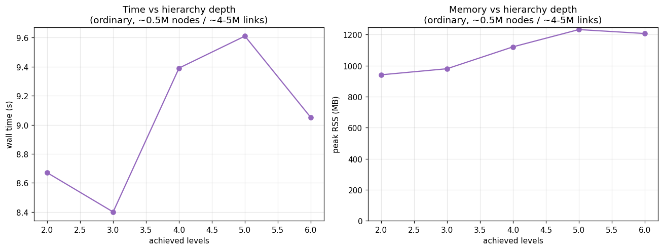
5. The cost of hierarchy depth

At a fixed size, time and memory rise with the number of levels Infomap recovers. You don’t choose depth; it follows from your network’s structure. That is why two networks of similar size can have different footprints, and why deep networks are the ones that gain from threads (§2) and --two-level (§4).

d = blk("B4b").dropna(subset=["levels"]).sort_values("levels")
fig, (ax1, ax2) = plt.subplots(1, 2, figsize=(12, 4.6))
ax1.plot(d.levels, d.wall_s, "o-", color="#9467bd")
ax2.plot(d.levels, d.peak_rss_mb, "o-", color="#9467bd")
_sub = "ordinary, ~0.5M nodes / ~4-5M links"
ax1.set_xlabel("achieved levels")
ax1.set_ylabel("wall time (s)")
ax1.set_title(f"Time vs hierarchy depth\n({_sub})")
ax2.set_xlabel("achieved levels")
ax2.set_ylabel("peak RSS (MB)")
ax2.set_title(f"Memory vs hierarchy depth\n({_sub})")
ax2.set_ylim(bottom=0)
plt.tight_layout()
plt.show()

6. Realistic anchor runs

The table below lists full end-to-end runs you can compare your own case against.

anchors = blk("B5").copy()
labelmap = {
    "a_ord1M_N1_t1": "ordinary 1M, 1 trial, 1 thread",
    "a_ord5M_N10_t10": "ordinary 5M, 10 trials, 10 threads",
    "a_ord20M_N10_t10": "ordinary 20M, 10 trials, 10 threads",
    "a_state1M_N10_t10": "state 1M, 10 trials, 10 threads",
    "a_state5M_N10_t10": "state 5M, 10 trials, 10 threads",
    "a_ml2M_N1_t8": "multilayer 2M, 1 trial, 8 threads",
}
anchors["case"] = anchors.label.map(labelmap)
order = list(labelmap.values())
tab = (
    anchors.set_index("case")
    .loc[order, ["wall_s", "GB"]]
    .rename(columns={"wall_s": "wall time (s)", "GB": "peak RSS (GB)"})
    .round(2)
)
tab

	wall time (s)	peak RSS (GB)
case
ordinary 1M, 1 trial, 1 thread	2.50	0.24
ordinary 5M, 10 trials, 10 threads	85.18	1.22
ordinary 20M, 10 trials, 10 threads	433.26	2.86
state 1M, 10 trials, 10 threads	30.52	0.38
state 5M, 10 trials, 10 threads	180.78	1.79
multilayer 2M, 1 trial, 8 threads	30.92	1.12

Estimating your own run

1. Count your links L and identify the type (ordinary, state, or multilayer).

2. Memory: peak RSS ≈ L × bytes-per-link from §1 (about 250 B ordinary, 370 B state, 600 B multilayer). Confirm it fits your RAM with headroom.

3. Time: for one trial on about 8 threads, ≈ L ÷ throughput from §1 (about 0.35M/s ordinary, 0.22M/s state, 0.06M/s multilayer). Multiply by your trial count.

4. Threads: use up to 8. They help a deep hierarchy (about 2.5×) and barely help a flat one, so don’t expect a linear speedup and don’t count on the efficiency cores.

5. Trials: a linear time cost with no extra memory, so budget N × one-trial time.

6. --two-level: if you only need communities, or a deep network is straining your memory, it runs about 1.5× faster and 30% lighter.

These come from one machine, so use them as ratios and anchor points, then calibrate with one small run of your own (or re-run with RUN_BENCHMARK = True).

For what these options do, see the options guide; for a first run, see the quickstart.