Temporal networks

Flow model

At a glance

Model time-varying interactions as one layer per snapshot, let inter-layer coupling carry community identity across time, and let Infomap reveal how groups change from one window to the next.

Communities that come and go

Most real interaction data have a timestamp. Friendship ties strengthen and dissolve, and researchers switch between fields. A static graph that aggregates all those interactions collapses the dynamics into a single picture and hides the change.

In a temporal network you instead get a sequence of snapshots, one per time window, and the question shifts from “which nodes form communities?” to “how do those communities evolve?” A cluster of colleagues who meet every morning and disperse at noon differs from a cluster that meets every day.

The cost of ignoring time is that naive approaches miss intermittent communities: groups that form, dissolve, and re-form in a recurring pattern. Face-to-face contact networks make this concrete: workplace social groups recur daily on a timescale of tens of minutes, but uniform aggregation smears them into background noise [Aslak et al., 2018]. Recovering that intermittent structure takes a model that couples information across time while respecting the boundaries between distinct interaction contexts.

Infomap handles temporal networks through the multilayer representation: you give each time window its own layer, connect a node’s copies across layers with inter-layer transitions, and run the standard map equation optimisation. The multilayer coding scheme tracks physical identity across layers, so a node that stays in the same community across several time windows receives consistent module labels. Later work [Holmgren et al., 2023] extended this to visualise how modular structure changes between snapshots, including alluvial diagrams that show modules merging and splitting over time.

Layers as time windows

Picture six colleagues. In the morning (T = 1) they split into two coffee-break groups: {Alice, Bob, Carol} and {Dave, Eve, Frank}. At midday (T = 2) the project teams shuffle: {Alice, Bob, Dave} work on one task while {Carol, Eve, Frank} handle another. By the afternoon (T = 3) the original coffee-break groups reconvene.

If you aggregate all interactions across the day into one static graph, every node connects to every other and the modular structure dissolves. If you treat each time window as a separate layer and let a random walker jump between layers with some probability, Infomap can follow the communities as they shift. Nodes that are consistently co-grouped across time share more flow, and the map equation finds the partition that best compresses that multi-window journey.

The strength of that coupling is set by the inter-layer relax rate \(r\); Multilayer networks describes the mechanism.

Coupling snapshots across time

A temporal network is a multilayer network whose layers are time windows: each node gets one state node per window, intra-layer links connect state nodes within a snapshot, and an inter-layer relax rate \(r\) carries the walker (and with it community identity) across windows. The multilayer chapter covers that machinery, including the relax-rate transition probabilities and how state nodes of one physical node share a codeword within a module. What is specific to time is how the windows should be coupled.

Uniform relaxation (the default) lets the walker relax to any window, weighted only by the node’s link strength there, and no window is privileged over another. It is the simplest choice and works well when communities change gradually.

Neighbourhood flow coupling (multilayer_relax_by_jsd) makes the coupling proportional to the Jensen-Shannon similarity (one minus the divergence) between a node’s link patterns in two windows, so windows where its context looks similar couple strongly. This matters for intermittent communities (groups that appear, vanish, and reappear), where coupling every window together would merge distinct occurrences that happen to share nodes [Aslak et al., 2018].

multilayer_relax_limit enforces temporal ordering: it caps how far the walker may relax in layer index, so the walk crosses only into nearby time windows rather than jumping across the whole sequence.

Six colleagues over three windows

The example below builds a tiny temporal network with six nodes and three time windows to show how Infomap tracks communities as they drift.

Setup. The six nodes represent people. In window T = 1 and again in T = 3 they interact in two stable triangles: {1, 2, 3} and {4, 5, 6}. In window T = 2 the groups reshuffle: {1, 2, 4} form one cluster while {3, 5, 6} form another. Add each layer as intra-layer links and let Infomap generate the inter-layer transitions automatically using a relax rate of 0.25.

import infomap
import networkx as nx
import matplotlib.pyplot as plt
from infomap import Network, run
from docs_viz import draw_partition, module_palette

# Three time windows; (source, target) pairs active in each window.
#   T=1  morning   : two triangles: {1,2,3}   and {4,5,6}
#   T=2  midday    : groups shift: {1,2,4}   and {3,5,6}
#   T=3  afternoon : triangles back: {1,2,3}   and {4,5,6}
edges_by_layer = {
    1: [(1, 2), (2, 3), (3, 1), (4, 5), (5, 6), (6, 4)],
    2: [(1, 2), (2, 4), (4, 1), (3, 5), (5, 6), (6, 3)],
    3: [(1, 2), (2, 3), (3, 1), (4, 5), (5, 6), (6, 4)],
}

# Build the multilayer network.  One intra-layer link per active edge;
# Infomap generates inter-layer transitions from the relax rate.
net = Network()
for layer_id, edges in edges_by_layer.items():
    for u, v in edges:
        net.add_multilayer_intra_link(layer_id, u, v)

result = run(net, multilayer_relax_rate=0.25, silent=True, seed=123)
print(f"Top-level modules : {result.num_top_modules}")
print(f"Codelength        : {result.codelength:.4f} bits/step")

Top-level modules : 2
Codelength        : 2.1586 bits/step

Infomap finds two top-level modules, one per persistent community, and keeps that assignment stable across all three windows.

Now extract the per-layer module assignments from the state nodes:

# Build a per-layer lookup: layer_id -> {physical_node_id: module_id}
layer_modules = {}
for node in result.nodes(states=True):
    layer_modules.setdefault(node.layer_id, {})[node.node_id] = node.module_id

for t in sorted(layer_modules):
    print(f"Layer {t}: {dict(sorted(layer_modules[t].items()))}")

Layer 1: {1: 1, 2: 1, 3: 1, 4: 2, 5: 2, 6: 2}
Layer 2: {1: 1, 2: 1, 3: 2, 4: 1, 5: 2, 6: 2}
Layer 3: {1: 1, 2: 1, 3: 1, 4: 2, 5: 2, 6: 2}

The output shows the community drift: node 3 leaves its morning group at midday (T = 2), while node 4 temporarily joins that group, then both return to their original affiliations by afternoon (T = 3).

Finally, draw all three time windows side by side, with nodes coloured by module:

import matplotlib.pyplot as plt
from myst_nb import glue

fig, axes = plt.subplots(1, 3, figsize=(10, 3.5), layout="constrained")
titles = {1: "T = 1  (morning)", 2: "T = 2  (midday)", 3: "T = 3  (afternoon)"}

# One shared palette across all windows, so a community keeps its colour over
# time and the drift of nodes 3 and 4 is visible as a colour change.
colours = module_palette(
    m for t in (1, 2, 3) for m in layer_modules[t].values()
)

# Per-window flow, so a node's radius tracks how often the walk visits it then.
layer_flow = {}
for node in result.nodes(states=True):
    layer_flow.setdefault(node.layer_id, {})[node.node_id] = node.flow

for t, ax in zip([1, 2, 3], axes):
    G = nx.Graph()
    G.add_nodes_from(range(1, 7))
    G.add_edges_from(edges_by_layer[t])
    draw_partition(
        G, layer_modules[t], ax=ax, module_colors=colours,
        with_labels=True, node_size=500, flow=layer_flow[t],
    )
    ax.set_title(titles[t], fontsize=11)

fig.suptitle("Temporal communities across three time windows", fontsize=12)
glue("fig-temporal", fig, display=False)
plt.close(fig)

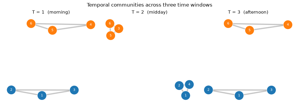
Fig. 11 One network per time window, coloured by community with a shared palette so a colour means the same community throughout. Nodes 3 and 4 swap colours at midday and return by afternoon: the community drift the multilayer coupling tracks.

Because the relax rate couples the layers, Infomap does not treat the T = 2 partition as independent: the same two underlying communities keep their module ids across all three windows instead of being assigned arbitrary new ones.

What the relax rate controls

Lowering multilayer_relax_rate toward zero makes each layer more autonomous, which helps when snapshots are far apart in time and you should not assume community identity persists. Raising it toward 1 pushes Infomap toward the aggregate static solution. The default is 0.15; values in the 0.15–0.25 range are usually a good choice for networks where communities evolve smoothly, and neighbourhood flow coupling stays robust across a broad range of relax rates (about 0.15 to 0.7) on their synthetic benchmarks [Aslak et al., 2018].

For long time series, multilayer_relax_limit caps how far the random walker may jump between layers, so coupling stays between temporally nearby windows rather than all pairs. Setting multilayer_relax_limit=1 confines coupling to the immediately neighbouring windows (layer index distance 1, in both directions), which suits ordered data such as geologic time series.

Visualising change over time

The side-by-side panels above suit small networks. For larger datasets with many modules and time steps, the standard MapEquation visualisation is an alluvial diagram, which tracks how modules merge and split across steps; the generator at https://www.mapequation.org/alluvial accepts Infomap output directly and generalises to higher-order and temporal networks [Holmgren et al., 2023].

API pointers

• infomap.Network.add_multilayer_intra_link() adds an edge within a single time-window layer: add_multilayer_intra_link(layer_id, source, target, weight=1.0).

• infomap.Network.add_multilayer_inter_link() adds an explicit inter-layer transition for a physical node: add_multilayer_inter_link(source_layer_id, node_id, target_layer_id, weight=1.0). Use it when you have empirical coupling weights; omit it to let Infomap generate transitions from multilayer_relax_rate.

• infomap.Network.add_multilayer_link() adds a fully specified multilayer link (layer, node) -> (layer, node) when you want complete control over the state-node graph.

• multilayer_relax_rate (an engine option on infomap.run()) sets the inter-layer relax rate \(r \in [0, 1]\) when you use add_multilayer_intra_link without explicit inter-layer links. 0.15–0.25 is a typical starting point.

• multilayer_relax_limit restricts relaxation to layers within a given index distance, enforcing temporal ordering.

• multilayer_relax_by_jsd=True uses neighbourhood flow coupling (Jensen-Shannon divergence) instead of uniform coupling; reach for it when communities are intermittent [Aslak et al., 2018].

• infomap.Result.nodes() with states=True iterates state nodes; each exposes .node_id, .layer_id, and .module_id to reconstruct per-layer community assignments.

• infomap.Result.modules() returns a {state_id: module_id} dict when called with states=True; use result.nodes(states=True) for the layer-aware view shown in the worked example.

Options

Temporal coupling is set by the multilayer engine options on infomap.run():

Option	Default	Effect
multilayer_relax_rate	0.15	Inter-layer coupling; higher couples windows more, toward the aggregate
multilayer_relax_limit	-1	Caps how far in layer index the walker may relax; enforces temporal ordering
multilayer_relax_by_jsd	False	Couple windows by neighbourhood-flow similarity instead of uniformly

Going deeper

• Aslak et al. [2018] introduce neighbourhood flow coupling and validate it on face-to-face contact networks.

• Alluvial diagrams for higher-order networks, with an interactive generator at https://www.mapequation.org/alluvial [Holmgren et al., 2023].

• The survey (§5.3) covers temporal networks and the multilayer representation [Smiljanić et al., 2026]; its companion notebook examples/notebooks/5.3 Modeling Temporal Data.ipynb discusses the Pajek format and the multilayer_relax_by_jsd option.