Networks with metadata

Flow model

At a glance

Node attributes (such as roles or categories) can guide community detection. The metadata map equation adds an attribute-homogeneity term to the description length, and a single rate parameter sets how much the attributes matter relative to the topology.

When attributes should guide clustering

Network topology alone does not always capture the communities you care about. Nodes carry attributes (the profession of a person in a social network, or the functional category of a protein), and those attributes may align with topological structure or cut across it. When they align, ignoring them throws away information you already have. When they cut across topology, you have to decide whether a community should be defined by where flow is trapped or by who shares a role.

Standard Infomap treats all nodes as identical; only the link weights influence the partition. You can annotate nodes with attributes in a post-processing step, but the partition itself never sees them. For attributes to influence the partition, they have to enter during community detection.

The metadata map equation [Emmons and Mucha, 2019] solves this by adding an attribute codebook term to the map equation. Encoding the random walk now requires encoding the attribute value at each step, and the extra cost is lower when modules are attribute-homogeneous. A tuning parameter \(\eta\), called meta_data_rate in the API, sets the relative weight of that attribute term. At \(\eta = 0\) you recover ordinary Infomap. As \(\eta\) grows you favour attribute-homogeneous modules more, accepting a longer topological description in return.

A closely related approach couples metadata to the map equation differently: it leaves the walk unchanged but makes the encoding of the walk depend on the metadata, which maps nonlocal relationships between attributes and network structure [Bassolas et al., 2022]. Both approaches capture the interplay between topology and metadata; the Emmons & Mucha formulation is what Infomap implements.

An attribute codebook

In the standard map equation, each module has a local codebook that names its nodes, and switching modules costs an inter-module codeword (The map equation). Now suppose each node also has a colour (its attribute) and you want modules where all nodes share a colour.

The metadata codebook adds a second layer of naming within each module: it also encodes the attribute value at every step. If a module holds nodes of one colour, the module name alone tells you the attribute, with no extra bits. If a module mixes colours, the encoder spends extra bits to say which colour appears at each step.

Raising \(\eta\) raises the cost of the attribute channel, which pushes the search toward homogeneous modules. The algorithm minimises the combined cost: topological compression plus attribute encoding. At low \(\eta\) the result looks like ordinary Infomap. At high \(\eta\) it looks more like grouping nodes by attribute, using topology only to settle borderline cases.

The metadata map equation

For a partition \(\mathsf{M}\) of \(n\) nodes into \(m\) modules and a set \(U\) of discrete attribute values, the metadata map equation from Emmons and Mucha [2019], Eq. 3, is:

\[ L_\eta(\mathsf{M}) = q_{\curvearrowright} H(\mathcal{Q}) + \sum_{i=1}^{m} p_{\circlearrowright}^i H(\mathcal{P}^i) + \eta \sum_{i=1}^{m} r_{\circlearrowright}^i H(\mathcal{R}^i) \]

The first two terms are the standard map equation: the inter-module codebook cost and the within-module codebook cost. The third term is new.

For module \(i\), let \(r_u^i = \sum_{\alpha \in i,\, u_\alpha = u} p_\alpha\) be the stationary flow through nodes with attribute \(u\), and \(r_{\circlearrowright}^i = \sum_{u} r_u^i\) the total flow through that module. The metadata entropy of module \(i\) is

\[ H(\mathcal{R}^i) = -\sum_{u \in U} \frac{r_u^i}{r_{\circlearrowright}^i} \log\!\left(\frac{r_u^i}{r_{\circlearrowright}^i}\right). \]

When every node in module \(i\) shares the same attribute value, \(H(\mathcal{R}^i) = 0\) and no extra bits are needed. When attributes are fully mixed, \(H(\mathcal{R}^i)\) is large. The parameter \(\eta\) weights how much this metadata entropy matters relative to the topological terms.

At \(\eta = 0\) the metadata term vanishes and \(L_0\) is the ordinary map equation. At \(\eta = 1\) the encoding assigns equal cost to the topological and attribute channels, the original content map equation of Smith et al. [2016]. For \(\eta > 1\) the attribute channel weighs more, pulling the partition toward attribute-homogeneous modules.

What \(\eta\) controls and when each regime is useful

The parameter \(\eta\) has an interpretation as a relative channel cost. Imagine two separate channels: one transmitting the topological part of the walk (module crossings, node names) and one transmitting the attribute value at each step. If accessing the attribute channel costs \(\eta\) times as much as the topological channel, then \(L_\eta\) is the total expected cost.

In practice the useful range of \(\eta\) is problem-dependent. Emmons and Mucha [2019] show that raising \(\eta\) (up to \(\eta = 1\) in their experiments) lets metadata push past the topological detectability limit when the attribute signal is strong but the topological signal is weak. Beyond \(\eta = 1\) the encoding increasingly enforces attribute-homogeneous modules, approaching the \(\eta \to \infty\) constrained limit where every module is attribute-pure.

The attribute codebook term encodes the metadata value at each step within the module. This is strictly more expensive than the topological encoding when modules are heterogeneous: a purely attribute-homogeneous partition where every module has exactly one attribute value incurs zero metadata cost in the third term, regardless of \(\eta\). The optimisation therefore pushes modules toward homogeneity as \(\eta\) increases, even splitting topologically tight groups if their attribute mixture is expensive to encode.

A complementary approach, metadata-dependent encoding of random walks [Bassolas et al., 2022], leaves the walk dynamics unchanged and instead makes the encoding of the walk depend on the metadata of the nodes the walker visits. That captures nonlocal relationships between metadata and network structure, rather than the local per-module codebook penalty used here. The two frameworks share a spirit but differ in where the metadata enters the encoding.

Two triangles, two attributes

The network below has six nodes arranged as two triangles connected by a bridge edge. Nodes 3 and 4, one in each triangle, share attribute category 1, while nodes 1, 2, 5, 6 share category 0.

Topologically, the bridge between node 3 and node 4 makes 3 and 4 the natural “boundary” between the two halves of the network, so pure topology puts {1, 2, 3} in one module and {4, 5, 6} in another. Each of those modules contains exactly one node with the minority attribute, so neither is attribute-homogeneous. With a non-zero meta_data_rate, the algorithm resolves the tension by splitting further, trading a longer topological description for attribute-pure modules.

Build the network and declare attributes

import infomap
import networkx as nx
from infomap import Network, run

# Two triangles joined by a bridge edge
G = nx.Graph()
G.add_edges_from([
    (1, 2), (1, 3), (2, 3),   # left triangle
    (3, 4),                     # bridge edge
    (4, 5), (4, 6), (5, 6),    # right triangle
])

# Node attributes: two categories
# Category 0: nodes 1, 2, 5, 6  (outer nodes in each triangle)
# Category 1: nodes 3, 4        (bridge-adjacent nodes)
metadata = {1: 0, 2: 0, 3: 1, 4: 1, 5: 0, 6: 0}

net = Network()
for u, v in G.edges():
    net.add_link(u, v)
for node_id, category in metadata.items():
    net.set_meta_data(node_id, category)

Topology only (rate = 0)

result_topo = run(net, meta_data_rate=0, silent=True, num_trials=10)
mods_topo = result_topo.modules()

print(f"Topology-only partition: {result_topo.num_top_modules} modules")
print(f"  Codelength: {result_topo.codelength:.4f} bits/step\n")

header = f"  {'node':>5}  {'module':>6}  {'attribute':>10}"
print(header)
print("  " + "-" * (len(header) - 2))
for nid in sorted(mods_topo):
    print(f"  {nid:>5}  {mods_topo[nid]:>6}  {metadata[nid]:>10}")

Topology-only partition: 2 modules
  Codelength: 2.3207 bits/step

   node  module   attribute
  -------------------------
      1       1           0
      2       1           0
      3       1           1
      4       2           1
      5       2           0
      6       2           0

At rate 0, Infomap finds the two topological communities: {1, 2, 3} and {4, 5, 6}. Each module mixes both attribute categories.

Metadata-aware (rate = 2)

result_meta = run(net, meta_data_rate=2.0, silent=True, num_trials=10)
mods_meta = result_meta.modules()

print(f"Metadata-aware partition: {result_meta.num_top_modules} modules")
print(f"  Codelength: {result_meta.codelength:.4f} bits/step\n")

header = f"  {'node':>5}  {'module':>6}  {'attribute':>10}"
print(header)
print("  " + "-" * (len(header) - 2))
for nid in sorted(mods_meta):
    print(f"  {nid:>5}  {mods_meta[nid]:>6}  {metadata[nid]:>10}")

Metadata-aware partition: 3 modules
  Codelength: 3.3378 bits/step

   node  module   attribute
  -------------------------
      1       1           0
      2       1           0
      3       2           1
      4       2           1
      5       3           0
      6       3           0

At rate 2, the partition shifts to three attribute-homogeneous modules: {1, 2} (attribute 0), {3, 4} (attribute 1), and {5, 6} (attribute 0). The bridge nodes 3 and 4 are now in their own module, grouped by shared attribute rather than by their position in the topology. The codelength is higher because a three-module topological description is less efficient, but the metadata encoding cost is zero: each module is attribute-pure.

Codelength goes up: is that wrong?

result.codelength reports the combined objective \(L_\eta\): the topological map-equation value plus \(\eta\) times the attribute term. It therefore rises with meta_data_rate even when the partition does not change at all, simply because the weighted attribute term grows, so the numbers are not comparable across rates. result.meta_entropy isolates the attribute term; the topological part is result.codelength - meta_data_rate * result.meta_entropy.

Sweeping the metadata rate

meta_data_rate (\(\eta\)) takes any non-negative value. Sweeping it shows the partition move from purely topological toward attribute-homogeneous:

# A fresh network for the sweep, so re-running does not invalidate `result_meta`
# above (reading a Result after its network runs again raises a stale-result error).
net_sweep = Network()
for u, v in G.edges():
    net_sweep.add_link(u, v)
for node_id, category in metadata.items():
    net_sweep.set_meta_data(node_id, category)

print(f"{'meta_data_rate':>14}  {'modules':>8}  {'codelength':>12}")
print("-" * 38)
for eta in [0.0, 0.5, 1.0, 2.0, 5.0]:
    r = run(net_sweep, meta_data_rate=eta, num_trials=10, seed=123, silent=True)
    print(f"{eta:>14.1f}  {r.num_top_modules:>8}  {r.codelength:>12.4f}")

meta_data_rate   modules    codelength
--------------------------------------
           0.0         2        2.3207
           0.5         2        2.8133
           1.0         2        3.3060
           2.0         3        3.3378
           5.0         3        3.3378

The module counts printed above show where the balance tips for this network.

Visualise the metadata-aware partition

import matplotlib.pyplot as plt
from myst_nb import glue

from docs_viz import draw_partition

flow = {n.node_id: n.flow for n in result_meta.nodes()}
fig = draw_partition(G, mods_meta, flow=flow)
glue("fig-metadata", fig, display=False)
plt.close(fig)

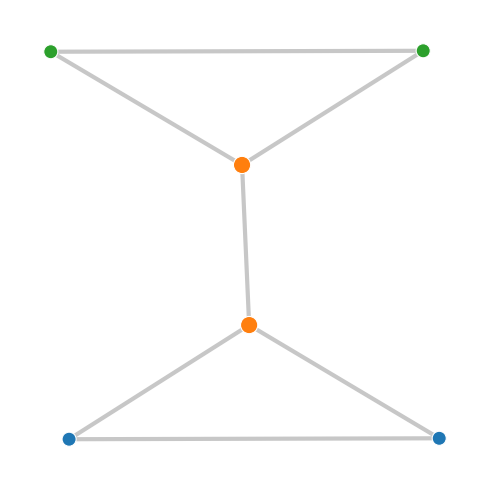
Fig. 12 The network coloured by the partition Infomap finds when node metadata is folded into the objective. A higher metadata rate trades a little topological compression for modules more homogeneous in the attribute.

The three attribute-homogeneous groups are visible: the two outer node pairs (one on each triangle) share the same attribute and land in separate modules, while the bridge pair {3, 4} forms its own cluster in the centre.

API pointers

• infomap.Network.set_meta_data() declares the attribute for a node: set_meta_data(node_id, meta_category). Each node takes one integer category label; call it once per node before the run.

• meta_data_rate (an engine option on infomap.run(), default 1.0; no effect unless you declare metadata) sets \(\eta\), the weight of the attribute codebook term. Pass meta_data_rate=0 to suppress all metadata influence.

• infomap.Result.meta_entropy is the metadata entropy term of the best partition, in bits per step.

Two further engine options:

• meta_data is a path to a metadata file listing node_id category pairs.

• meta_data_unweighted, when True, ignores node visit frequencies when computing the metadata codebook and treats all nodes as equally visited.

Options

Metadata influence is set by these engine options on infomap.run():

Option	Default	Effect
meta_data_rate	1.0	Weight \(\eta\) of the attribute codebook; 0 ignores metadata
meta_data_unweighted	False	Treat all nodes as equally visited in the metadata term
meta_data	None	Path to a node_id category file instead of set_meta_data

Going deeper

• Emmons and Mucha [2019] is the source paper Infomap implements; a related metadata-dependent random walk is developed in [Bassolas et al., 2022].

• The survey (§6.1) covers metadata-aware community detection [Smiljanić et al., 2026], with companion notebook examples/notebooks/6.1 Networks with Metadata.ipynb.