Reading Infomap through Louvain and Leiden

Concept

At a glance

If you already use Louvain or Leiden, you can read Infomap through the same lens: all three partition a network, but Infomap optimises the compression of flow where Louvain and Leiden optimise modularity.

Same job, a different objective

Louvain and Leiden are the community-detection methods most researchers meet first, and both return a partition of your nodes just as Infomap does. This page maps Infomap onto the concepts you already know from them.

The main difference is the objective. Louvain and Leiden score a partition by modularity: whether more edges fall inside groups than a random graph with the same degrees would predict. Infomap scores it by the map equation: how few bits describe a random walk on the network under that partition (see The map equation).

Running both is a useful sanity check. Where the two agree, the grouping is robust to the choice of objective; where they differ, the grouping depends on what you mean by “community”.

What each objective optimises

Modularity (Louvain, Leiden). Both are usually run to maximise modularity, a static-density score against a degree-preserving null model. Standard modularity’s null model is undirected, so edge direction is ignored unless you switch to a directed-modularity variant. Leiden is a general optimiser: it maximises whichever quality function you give it, adds a refinement step that guarantees internally connected communities, and reaches better optima than Louvain’s greedy moves [Traag et al., 2019]. This page uses the modularity objective for both, the most common default.

The map equation (Infomap). Infomap compresses a description of a random walk (see The map equation). A group is worth naming when a walker entering it tends to stay for several steps before leaving. Because the walk follows edge direction and weight, Infomap reads those where an undirected modularity null model does not.

Modularity and the map equation

Modularity for a partition \(\mathsf{C}\) is

\[ Q = \frac{1}{2m} \sum_{i,j} \left[ A_{ij} - \frac{k_i k_j}{2m} \right] \delta(c_i, c_j), \]

where \(A_{ij}\) is the adjacency matrix, \(k_i\) is degree, and \(m\) is the number of edges. The map equation \(L(\mathsf{M})\) is instead

\[ L(\mathsf{M}) = q_{\curvearrowright} H(\mathcal{Q}) + \sum_{i} p_{\circlearrowright}^i H(\mathcal{P}^i), \]

summed over the modules \(i\): the average cost of coding a random walk, bits for crossing module boundaries plus bits for moving inside them.

A note on the resolution limit

Modularity has a resolution limit: it tends not to separate communities with fewer than roughly \(\sqrt{m/2}\) internal links, however cohesive they are [Fortunato and Barthélemy, 2007]. Leiden can sidestep it with a resolution-limit-free objective such as the Constant Potts Model, or by tuning its resolution_parameter. The map equation has a resolution limit too, weaker but not absent (Hierarchy and the multilevel map equation derives the bound); tune its scale with markov_time or preferred_number_of_modules. These are properties of the objectives, not verdicts on them.

One network under each objective

Here is one clearly structured network partitioned by all three methods.

import networkx as nx
import infomap
import igraph as ig
import random

# Four well-separated groups by construction. Sampling with Python's `random`
# keeps the graph identical across NetworkX versions.
rng = random.Random(123)
n_groups, n_per = 4, 12
g = nx.Graph()
g.add_nodes_from(range(n_groups * n_per))
for i in range(n_groups * n_per):
    for j in range(i + 1, n_groups * n_per):
        p = 0.7 if i // n_per == j // n_per else 0.05
        if rng.random() < p:
            g.add_edge(i, j)

# Infomap: compress the flow
result = infomap.run(g, two_level=True, seed=123, num_trials=10, silent=True)
infomap_mods = result.modules()

# Louvain and Leiden: maximise modularity
louvain = nx.community.louvain_communities(g, seed=123)
louvain_mods = {n: c for c, comm in enumerate(louvain) for n in comm}

ig_g = ig.Graph(edges=list(g.edges()), n=g.number_of_nodes(), directed=False)
random.seed(123)  # python-igraph draws from the global RNG
leiden = ig_g.community_leiden(objective_function="modularity", n_iterations=10)
leiden_mods = {n: m for n, m in enumerate(leiden.membership)}

print(f"Infomap (flow):        {len(set(infomap_mods.values()))} groups")
print(f"Louvain (modularity):  {len(louvain)} groups")
print(f"Leiden  (modularity):  {len(leiden)} groups")

Infomap (flow):        4 groups
Louvain (modularity):  4 groups
Leiden  (modularity):  4 groups

import matplotlib.pyplot as plt
from myst_nb import glue
from docs_viz import draw_partition

fig, axes = plt.subplots(1, 3, figsize=(11, 3.6), layout="constrained")
for ax, (name, mods) in zip(
    axes,
    [("Infomap (flow)", infomap_mods),
     ("Louvain (modularity)", louvain_mods),
     ("Leiden (modularity)", leiden_mods)],
):
    draw_partition(g, mods, ax=ax)
    ax.set_title(name, fontsize=11)
fig.suptitle("The same network under each objective", fontsize=12)
glue("fig-choosing-a-method", fig, display=False)
plt.close(fig)

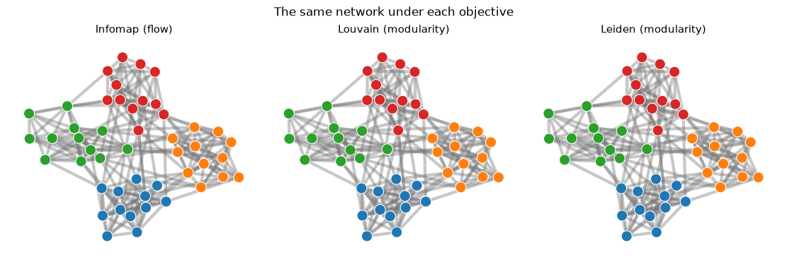
Fig. 5 One network partitioned by each objective; the group counts print above. Colours identify groups within a panel, not across panels.

On well-separated, undirected structure like this the two objectives agree, which is the common case: compressing the flow and maximising within-group density pick out the same groups.

Where the objectives differ

Infomap’s answer differs from a modularity partition in two situations:

• Directed flow. Infomap follows edge direction; the standard modularity null model does not. On a network with real flow asymmetry, a citation cascade or a web subgraph that mostly sends links one way, the random walk concentrates where undirected edge density alone does not, so a directed Infomap run reads the structure differently [Rosvall and Bergstrom, 2008].

• Scale. The two objectives have different resolution limits (see the toggle above), so on a network with many small groups they need not agree on how finely to divide it. Neither is more correct; they optimise different things.

These are the two places where “community by flow” and “community by density” genuinely mean different things; knowing your network tells you which to trust.

API pointers

• infomap.run() returns an immutable Result; pass directed=True for directed-flow treatment and two_level=True for a flat partition.

• infomap.find_communities() returns a NetworkX-style list[set], and infomap.find_igraph_communities() returns an igraph.VertexClustering, so an Infomap result plugs into igraph’s own inspection and plotting utilities alongside Louvain and Leiden.

Going deeper

• The map equation derives why Infomap minimises description length rather than maximising modularity.

• Companion notebooks: examples/notebooks/compare-infomap-louvain-networkx.ipynb and examples/notebooks/compare-infomap-louvain-leiden-igraph.ipynb show the side-by-side workflow with NetworkX and igraph.

• Traag et al. [2019] introduces Leiden and shows Louvain can return internally disconnected communities.

• Fortunato and Barthélemy [2007] is the original proof of modularity’s resolution limit.

• The map equation versus modularity on flow and non-flow networks [Rosvall and Bergstrom, 2008].

• The survey (§3) treats the two objectives side by side [Smiljanić et al., 2026].