Multilayer networks¶
Flow model
At a glance
A multilayer network lets the same physical node live in several layers at once, so Infomap can discover that a person belongs to one community at work and a different one at home, without collapsing those contexts into one network.
Why aggregating layers loses structure¶
Many real systems involve the same actors interacting through several kinds of relationship at once: scientists collaborate on papers and correspond by email, passengers fly between airports on different airlines. Collapse the interaction types into one network and you lose the contextual information that defines who belongs to which community in each setting.
A multilayer network preserves those contexts by keeping each interaction type in its own layer. The same physical entity exists in each layer where it participates, but its neighbourhood and community membership can differ from layer to layer. Aggregating the layers into one network can distort both the topology and the community structure [De Domenico et al., 2015].
Multilayer networks also express overlapping communities: because the same physical entity lives in several layers, Infomap can place it in a different module in each. The next sections show the mechanism.
One node, several layers¶
Think of a research collaboration network. Layer 1 records co-authorship on machine-learning papers; Layer 2 records co-authorship on statistics papers. Researcher Alice publishes in both fields. Her Layer-1 state node connects to her ML co-authors, her Layer-2 state node to her statistics co-authors. Those are two different neighbourhoods.
Infomap runs a random walk across all the state nodes. The walk stays in its current layer most of the time and crosses to another at rate \(r\), the relax rate. When it rarely crosses (\(r\) small), each layer behaves on its own and Alice lands in a different module in each of her layers. When it crosses freely (\(r = 1\)), the layers fuse and Alice gets one module. The default \(r = 0.15\) relaxes the layer constraint about once in seven steps (the relaxed step can land back in the current layer, so actual switches are rarer), enough coupling to respect the multiplex structure without washing out the per-layer signal.
The key step is that here a state node is a physical node’s presence in one layer; the rest of the physical-node/state-node mechanism is generic (State nodes and higher-order flow). A physical node that lands in two modules is thus bi-modular, with a flow signature that differs by layer [Edler et al., 2017].
State nodes and the relax rate¶
A multilayer network has \(L\) layers over a shared set of physical nodes. Each physical node \(i\) in layer \(\alpha\) becomes a state node \((i, \alpha)\). Links within a layer (intra-layer) connect state nodes in the same layer; links across layers (inter-layer) connect state nodes in different layers.
Without empirical inter-layer link weights, Infomap models inter-layer movement with a relax rate \(r \in [0, 1]\). At each step, the random walker follows intra-layer links with probability \(1 - r\) and relaxes the layer constraint with probability \(r\), freely following any link of the physical node across all layers:
where \(s_i^{\beta}\) is the intra-layer out-strength of node \(i\) in layer \(\beta\), and \(S_i = \sum_\beta s_i^\beta\) is the total out-strength across all layers. Setting \(r = 0\) decouples layers completely; \(r = 1\) is equivalent to running Infomap on the aggregated single-layer network (but still allowing overlap).
The relax-rate walk above runs over these state nodes; when \((i, \alpha)\) and \((i, \beta)\) split across modules, physical node \(i\) is bi-modular — the generic overlap mechanism of State nodes and higher-order flow.
State node transition probabilities (full derivation)
A multilayer network is a set of state nodes \(\{(i, \alpha)\}\) with intra-layer link weights \(w_{ij}^\alpha\) (both \(i\) and \(j\) in layer \(\alpha\)) and inter-layer link weights \(D_i^{\alpha\beta}\) (physical node \(i\) from layer \(\alpha\) to layer \(\beta\)). The general transition probability is
where \(S_i^\alpha = \sum_\beta D_i^{\alpha\beta}\) is the inter-layer out-strength of node \(i\) from layer \(\alpha\).
When no empirical inter-layer data are available, setting \(D_i^{\alpha\beta} = (1-r)\delta_{\alpha\beta}S_i + r\,s_i^\beta\) recovers the relax-rate formula above [De Domenico et al., 2015], with the default \(r = 0.15\) interpreted as in the narrative introduction.
The map equation then minimises
over partitions of state nodes into modules, where the map equation sums the visit rates of the same physical node in the same module before computing the module codebook entropy \(H(\mathcal{P}^{\boldsymbol{\imath}})\). As in State nodes and higher-order flow, this state-node aggregation is the sole change from the first-order map equation [De Domenico et al., 2015, Edler et al., 2017].
Two triangles bridged by one node¶
The network is the example the
multilayer input format
is documented with on mapequation.org (it ships with Infomap as
examples/networks/multilayer.net): five physical nodes i, j, k,
l, m in two layers.
Layer 1 contains a tight triangle: i, l, m.
Layer 2 contains a tight triangle: i, j, k.
Physical node i is the bridge: it participates in both layers. With a low relax rate, the map equation finds two modules, {i, l, m} from Layer 1 and {i, j, k} from Layer 2. Node i is bi-modular: one module per layer.
import infomap
from infomap import Network, Options, run

names = {1: "i", 2: "j", 3: "k", 4: "l", 5: "m"}

# (layer, source, target, weight): i sends weight 0.8 to its triangle
# partners and receives weight 1.0 back; the partners link with weight 1.0.
intra_links = [
    (1, 1, 4, 0.8), (1, 4, 1, 1.0), (1, 1, 5, 0.8), (1, 5, 1, 1.0),
    (1, 4, 5, 1.0), (1, 5, 4, 1.0),
    (2, 1, 2, 0.8), (2, 2, 1, 1.0), (2, 1, 3, 0.8), (2, 3, 1, 1.0),
    (2, 2, 3, 1.0), (2, 3, 2, 1.0),
]

net = Network()
for layer, src, tgt, w in intra_links:
    net.add_multilayer_intra_link(layer, src, tgt, w)

result = run(net, options=Options(multilayer_relax_rate=0.15), seed=123, num_trials=10)

state_nodes = list(result.nodes(states=True))
print(f"Modules found : {result.num_top_modules}")
print(f"Codelength    : {result.codelength:.4f} bits")
print(f"Physical nodes: {len({n.node_id for n in state_nodes})}")
print(f"State nodes   : {len(state_nodes)}")

# Guard the example: the discussion assumes two modules and a bi-modular i.
assert result.num_top_modules == 2
assert len({n.module_id for n in state_nodes if n.node_id == 1}) == 2
Modules found : 2
Codelength    : 1.7739 bits
Physical nodes: 5
State nodes   : 6
Infomap operates on six state nodes (one per physical-node–layer pair) and finds two modules. Now inspect the per-state-node partition to see the overlap:
print(f"{'Layer':>6}  {'Phys node':>10}  {'Module':>8}")
print("-" * 30)
for node in sorted(result.nodes(states=True), key=lambda n: (n.layer_id, n.node_id)):
    print(f"{node.layer_id:>6}  {names[node.node_id]:>10}  {node.module_id:>8}")
 Layer   Phys node    Module
------------------------------
     1           i         1
     1           l         1
     1           m         1
     2           i         2
     2           j         2
     2           k         2
Physical node i appears twice, once in each layer, in a different module each time. Nodes l and m sit only in the Layer 1 triangle’s module, nodes j and k only in the Layer 2 triangle’s module; the table above shows the module ids.
On multilayer networks you must call result.modules(states=True), because each
physical node can belong to multiple modules:
state_modules = result.modules(states=True)
print("state_id -> module_id:", state_modules)
state_id -> module_id: {0: 1, 1: 1, 2: 1, 3: 2, 4: 2, 5: 2}
You can recover the full per-layer picture from result.nodes(states=True):
from collections import defaultdict

# physical node -> list of (layer, module) pairs
phys_memberships = defaultdict(list)
for node in result.nodes(states=True):
    phys_memberships[node.node_id].append((node.layer_id, node.module_id))

print(f"{'Phys node':>10}  {'(layer, module) assignments'}")
print("-" * 45)
for pid, assignments in sorted(phys_memberships.items()):
    print(f"{names[pid]:>10}  {sorted(assignments)}")
 Phys node  (layer, module) assignments
---------------------------------------------
         i  [(1, 1), (2, 2)]
         j  [(2, 2)]
         k  [(2, 2)]
         l  [(1, 1)]
         m  [(1, 1)]
Physical node i has two assignments; all others have one.
Now draw both layers side by side, colouring each node by the module it lands in. A shared palette and a shared layout fix each module’s colour and node i’s position across panels, so i sits in the same spot in a different colour in each layer.
from myst_nb import glue

import matplotlib.pyplot as plt
import networkx as nx
from docs_viz import draw_partition, module_palette

# Layer triangles, and one shared layout: node i sits at the same spot (bottom
# centre) in both panels, and each layer's two partners take the same upper
# corners, so only colour and labels change between the panels.
layer_edges = {
    1: [("i", "l"), ("l", "m"), ("i", "m")],
    2: [("i", "j"), ("j", "k"), ("i", "k")],
}
pos = {"i": (0.0, -0.75),
       "l": (-0.95, 0.6), "m": (0.95, 0.6),
       "j": (-0.95, 0.6), "k": (0.95, 0.6)}

# Module assignment and flow per physical node, recorded separately per layer.
state_nodes = list(result.nodes(states=True))
module_in_layer = {
    layer: {names[n.node_id]: n.module_id for n in state_nodes if n.layer_id == layer}
    for layer in (1, 2)
}
flow_in_layer = {
    layer: {names[n.node_id]: n.flow for n in state_nodes if n.layer_id == layer}
    for layer in (1, 2)
}
colours = module_palette(
    m for layer in (1, 2) for m in module_in_layer[layer].values()
)

fig, axes = plt.subplots(1, 2, figsize=(8, 4), layout="constrained")
for ax, layer in zip(axes, (1, 2)):
    G = nx.Graph()
    G.add_edges_from(layer_edges[layer])
    draw_partition(
        G, module_in_layer[layer], ax=ax, module_colors=colours,
        with_labels=True, node_size=650, flow=flow_in_layer[layer],
        pos={n: pos[n] for n in G},
    )
    ax.set_title(f"Layer {layer}", fontsize=11)
    ax.set_xlim(-1.4, 1.4)
    ax.set_ylim(-1.15, 1.0)

fig.suptitle(
    "Physical node i is the bridge: the same node, a different module per layer",
    fontsize=12,
)
glue("fig-multilayer", fig, display=False)
plt.close(fig)
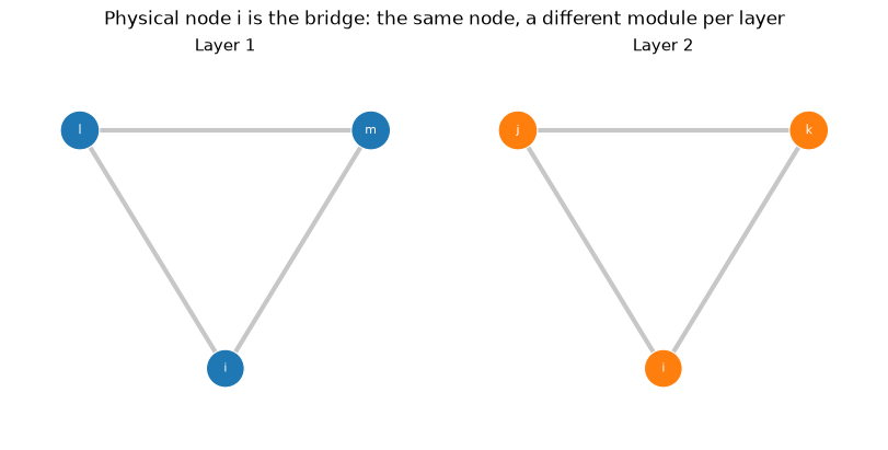
Fig. 10 The two layers drawn with one shared layout, coloured by module. Physical node i holds the same position in both panels but takes a different colour: the bi-modular overlap that state nodes make possible.¶
Relax rate sensitivity¶
The relax rate controls how strongly the layers couple. Low values treat each layer nearly independently; high values merge them into a single partition.
results = []
for r in [0.01, 0.15, 0.50, 0.90, 1.00]:
    net_r = Network()
    for layer, src, tgt, w in intra_links:
        net_r.add_multilayer_intra_link(layer, src, tgt, w)
    result_r = run(net_r, options=Options(multilayer_relax_rate=r), seed=123, num_trials=10)
    results.append((r, result_r.num_top_modules, result_r.codelength))

print(f"{'relax rate':>12}  {'modules':>8}  {'codelength':>12}")
print("-" * 36)
for r, m, cl in results:
    print(f"{r:>12.2f}  {m:>8}  {cl:>12.4f}")
  relax rate   modules    codelength
------------------------------------
        0.01         2        1.6034
        0.15         2        1.7739
        0.50         2        2.0791
        0.90         1        2.2636
        1.00         1        2.2636
At low relax rates the two triangle clusters remain distinct (2 modules). As \(r \to 1\) the layers fuse and the partition collapses to 1 module, the same as running Infomap on the aggregated network. The default \(r = 0.15\) is the working value from De Domenico et al. [2015], who found the partition only weakly dependent on the relax rate; later work confirmed that the partition stays robust across empirical multilayer networks for relax rates up to about \(r \approx 0.25\) [Edler et al., 2017].
Node-aligned inter-layer links¶
When the observed coupling is a node switching layer “in place” (a person
moving between the work and family contexts, a passenger changing airline at
the same airport), supply node-aligned inter-layer links with
add_multilayer_inter_link instead of relying on the relax-rate model. This
is the *Intra/*Inter file form, and the bundled
infomap.datasets.multilayer_intra_inter() network is its reference
example: the same two triangles, with an inter-layer link through i in each
direction. The transition happens at i; the flow it carries continues to
i’s neighbours in the target layer.
net_aligned = Network()

# Intra-layer links (same as before)
for layer, src, tgt, w in intra_links:
    net_aligned.add_multilayer_intra_link(layer, src, tgt, w)

# i switches layer in place: one inter-layer link through i each way.
net_aligned.add_multilayer_inter_link(1, 1, 2, 0.4)
net_aligned.add_multilayer_inter_link(2, 1, 1, 0.4)

result_aligned = run(net_aligned, seed=123, num_trials=10)
print(f"Modules found : {result_aligned.num_top_modules}")
print(f"Codelength    : {result_aligned.codelength:.4f} bits")

# The same construction ships with the package; the two must agree exactly.
result_pkg = infomap.run(infomap.datasets.multilayer_intra_inter(),
                         seed=123, num_trials=10)
assert result_aligned.codelength == result_pkg.codelength
Modules found : 2
Codelength    : 1.9734 bits
Fully explicit links¶
The most general form gives every link as a (layer, node) pair with
add_multilayer_link, including inter-layer links between different
physical nodes. This is the *Multilayer file form, and
infomap.datasets.multilayer() is its reference example: the twelve
intra-layer links from before plus four inter-layer links, from i to the
other layer’s triangle partners.
net_full = Network()

for layer, src, tgt, w in intra_links:
    net_full.add_multilayer_link((layer, src), (layer, tgt), w)

inter_links = [
    ((1, 1), (2, 2), 0.2),  # i in layer 1 -> j in layer 2
    ((1, 1), (2, 3), 0.2),  # i in layer 1 -> k in layer 2
    ((2, 1), (1, 4), 0.2),  # i in layer 2 -> l in layer 1
    ((2, 1), (1, 5), 0.2),  # i in layer 2 -> m in layer 1
]
for src, tgt, w in inter_links:
    net_full.add_multilayer_link(src, tgt, w)

result_full = run(net_full, seed=123, num_trials=10)
print(f"Modules found : {result_full.num_top_modules}")
print(f"Codelength    : {result_full.codelength:.4f} bits")

result_pkg = infomap.run(infomap.datasets.multilayer(),
                         seed=123, num_trials=10)
assert result_full.codelength == result_pkg.codelength
Modules found : 2
Codelength    : 2.0114 bits
When you provide explicit inter-layer links, Infomap does not use the relax-rate
model; the link weights you supply fully specify the coupling. The two
construction forms take different paths, however: the typed
add_multilayer_intra_link/add_multilayer_inter_link methods build per-layer
networks that Infomap expands, while add_multilayer_link writes state-level
links directly. Mixing them in one network does not reproduce the file form;
pick one form per network.
Relaxing to the same node only¶
Back in the relax-rate model, multilayer_relax_to_self=True links a relaxing
state node to its own physical node in the target layer instead of spreading
directly to its out-neighbours there. It shrinks the state network, which
matters on large networks. For a coherent partition the flow is unchanged; it
can differ slightly only when a node’s target-layer neighbours split across
modules:
net_self = Network()
for layer, src, tgt, w in intra_links:
    net_self.add_multilayer_intra_link(layer, src, tgt, w)

result_self = run(net_self,
                  options=Options(multilayer_relax_rate=0.15,
                                  multilayer_relax_to_self=True),
                  seed=123, num_trials=10)

n_links_self = len(list(result_self.links()))
n_links_default = len(list(result.links()))
print(f"Modules found: {result_self.num_top_modules}")
print(f"Codelength   : {result_self.codelength:.4f} bits")
print(f"State links  : {n_links_self} (vs {n_links_default} without the flag)")

# Same flow, smaller state network.
assert abs(result_self.codelength - result.codelength) < 1e-10
assert n_links_self < n_links_default
Modules found: 2
Codelength   : 1.7739 bits
State links  : 14 (vs 16 without the flag)
API pointers¶
Build multilayer input with
add_multilayer_intra_link(),add_multilayer_inter_link(), and the fully generaladd_multilayer_link()(all used above), or load a bundled example withmultilayer(),multilayer_intra(), andmultilayer_intra_inter().Read a multilayer run with
modules()/nodes()passingstates=True—states=Falseraises anInfomapErroron higher-order networks. Each state node carries.node_id(physical),.state_id,.layer_id,.module_id, and.flow.
Options¶
The relax-rate model is controlled by these engine options, carried via Options
to infomap.run() (options=Options(...)).
They apply when Infomap simulates the coupling; with explicit inter-layer links
only multilayer_relax_to_self still has an effect, deciding whether a
node-aligned inter link attaches to the node’s own copy or spreads over its
out-neighbours in the target layer:
Option |
Default |
Effect |
|---|---|---|
|
|
Probability per step of relaxing to another layer |
|
|
Relax only to layers at most this many layer ids away ( |
|
|
The same cap, counting only towards higher layer ids |
|
|
The same cap, counting only towards lower layer ids |
|
|
Weight relaxation by neighbourhood similarity; see Temporal networks |
|
|
Relax to the node’s own copy in the target layer instead of spreading to its out-neighbours; smaller state network, identical flow for coherent partitions |
Going deeper¶
Source paper for multilayer flows [De Domenico et al., 2015]; the higher-order treatment in Infomap follows [Edler et al., 2017].
The survey (§5.2) covers multilayer networks [Smiljanić et al., 2026], with companion notebook
examples/notebooks/5.2 Multilayer Networks.ipynb.