State nodes and higher-order flow¶

Concept

At a glance

A state node lets one real-world node carry several flow contexts at once. It is the mechanism behind memory, multilayer, and temporal networks, and it lets a node belong to more than one community.

When first-order flow is too simple¶

The map equation in the previous chapters assumes first-order flow: where the walker goes next depends only on where it is now. That is often too simple. Where a traveller flies next depends on where they came from, and which colleagues a person interacts with depends on the setting (work, home, a conference). Collapsing that context into a plain network averages it away.

The fix is to stop treating a node as a single thing. Memory, multilayer, and temporal networks all rest on the same construction, the state node, with different notions of “context.”

Physical nodes vs state nodes¶

Separate two ideas that an ordinary network conflates:

a physical node is the real-world object: an airport, a person, a paper;
a state node is that object in one context: “Chicago, arrived from Seattle”; “Alice, at work”; “this paper, in 2021.”

Infomap runs its random walk over the state nodes, and the map equation partitions those. The only change from the first-order map equation is that state nodes belonging to the same physical node within the same module share a codeword, because they are the same object.

If a physical node’s state nodes land in different modules, that physical node belongs to several communities at once, with no separate overlapping-community algorithm. Alice-at-work and Alice-at-home can sit in different groups, and a hub airport can belong to several regional systems.

The map equation on state nodes¶

A higher-order network is a set of state nodes, each attached to a physical node, with transitions between them. The map equation is unchanged in form (the sum still runs over the \(m\) modules),

\[ L(\mathsf{M}) = q_{\curvearrowright} H(\mathcal{Q}) + \sum_{i=1}^{m} p_{\circlearrowright}^i H(\mathcal{P}^i), \]

but it runs over state nodes: the map equation sums the visit rates of state nodes of the same physical node in the same module before computing the module codebook entropy.

One physical node in two modules¶

The classic illustration is the network that documents the states input format on mapequation.org (it ships with Infomap as examples/networks/states.net). It has five physical nodes i, j, k, l, m, where i carries two state nodes: from state \(\alpha_i\) the walker mostly continues to j and k, from state \(\delta_i\) mostly to l and m. The weak 0.2-links let it occasionally switch sides, so the two contexts are coupled but distinct.

Build state nodes directly with add_state_node(state_id, node_id), where node_id is the physical node, link them with add_link, then read the partition back with result.nodes(states=True):

import infomap
from infomap import Network, run

state_names = {1: "α", 2: "β", 3: "γ", 4: "δ", 5: "ε", 6: "ζ"}
phys_names = {1: "i", 2: "j", 3: "k", 4: "l", 5: "m"}

net = Network()
for state, phys in [(1, 1), (2, 2), (3, 3), (4, 1), (5, 4), (6, 5)]:
    net.add_state_node(state, phys)

links = [
    (1, 2, 0.8), (1, 3, 0.8), (1, 5, 0.2), (1, 6, 0.2),  # α: mostly to j, k
    (2, 1, 1.0), (2, 3, 1.0), (3, 1, 1.0), (3, 2, 1.0),
    (4, 5, 0.8), (4, 6, 0.8), (4, 2, 0.2), (4, 3, 0.2),  # δ: mostly to l, m
    (5, 4, 1.0), (5, 6, 1.0), (6, 4, 1.0), (6, 5, 1.0),
]
for src, tgt, w in links:
    net.add_link(src, tgt, w)

result = run(net, two_level=True, directed=True, seed=123, num_trials=10, silent=True)

print(f"Modules: {result.num_top_modules}")
for node in sorted(result.nodes(states=True), key=lambda n: n.state_id):
    name = f"{state_names[node.state_id]} (physical {phys_names[node.node_id]})"
    print(f"  state {name}: module {node.module_id}")

# The prose below relies on this structure; fail the build if it drifts.
mods_of_i = {n.module_id for n in result.nodes(states=True) if n.node_id == 1}
assert result.num_top_modules == 2 and len(mods_of_i) == 2

Modules: 2
  state α (physical i): module 1
  state β (physical j): module 1
  state γ (physical k): module 1
  state δ (physical i): module 2
  state ε (physical l): module 2
  state ζ (physical m): module 2

Physical node i appears in both modules, through \(\alpha_i\) on the j–k side and \(\delta_i\) on the l–m side. Every other node sits in one module.

Draw the state-level network, colouring each state node by the module Infomap assigned it:

import matplotlib.pyplot as plt
import networkx as nx
from docs_viz import draw_partition
from myst_nb import glue

g = nx.Graph()
for src, tgt, w in links:
    g.add_edge(state_names[src], state_names[tgt], weight=w)

# Colour each state node by its module; size it by its flow.
state_module = {state_names[n.state_id]: n.module_id for n in result.nodes(states=True)}
state_flow = {state_names[n.state_id]: n.flow for n in result.nodes(states=True)}

fig = draw_partition(g, state_module, with_labels=True, node_size=600, flow=state_flow)
glue("fig-state-nodes", fig, display=False)
plt.close(fig)

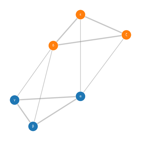
../_images/4764674eaa59d57613ff6e4f44021ae6029d462ce7bcfb3f5724cef7fed01f91.png — Fig. 4 The states-format example network, coloured by module. States α and δ are physical node i in its two contexts; they land in different modules, so i belongs to both. The figure shows the undirected skeleton; the walk itself follows the weighted, directed links.¶

The same network ships with the package¶

The construction above is the states-format reference example, so it comes bundled: infomap.datasets.states() returns it as a ready-to-run Network, loaded from the same .net file that documents the *States format (each state declared as state_id physical_id [name], with *Links connecting state ids). Running it reproduces the partition above exactly:

net_pkg = infomap.datasets.states()
result_pkg = infomap.run(net_pkg, two_level=True, directed=True,
                         seed=123, num_trials=10, silent=True)

print(f"Modules: {result_pkg.num_top_modules}, "
      f"codelength {result_pkg.codelength:.4f} bits per step")

# Same network, same partition as the construction above.
assert result_pkg.codelength == result.codelength

Modules: 2, codelength 2.0114 bits per step

Where this goes next¶

Each Flow models chapter is this idea with a specific kind of context:

Memory and state networks: context is where you came from.
Multilayer networks: context is which layer (relationship type).
Temporal networks: context is which time window.

They build the state nodes through higher-level APIs (add_multilayer_intra_link, time-window layers) rather than add_state_node directly, but the partition you read back is always over state nodes.

API pointers¶

Network().add_state_node(state_id, node_id) declares a state node on the physical node node_id; add_link then links state nodes.
You need result.modules(states=True) to read a higher-order partition; result.nodes(states=True) exposes each node’s .node_id (physical), .state_id, .module_id, and .flow.
result.have_memory is True once a higher-order network is built.

Going deeper¶

Edler et al. [2017] develop higher-order flows in memory and multilayer networks with Infomap.
The survey (§5) treats higher-order flow and state nodes in full [Smiljanić et al., 2026].