The map equation¶
Concept
At a glance
The map equation measures how many bits it takes to describe a random walk on your network. That number is the codelength; Infomap finds the partition that makes it smallest, which is the partition where flow stays trapped in modules.
Two questions you can ask of a network¶
When you split a network into communities, how do you know the split is good? You need a quality function: a single number that scores any candidate partition.
Many methods use modularity, which counts whether more edges fall inside modules than a random baseline would predict. Modularity asks how the network was wired.
The map equation asks how it is used. Given that flow moves through the network, say passengers through airports or clicks across the web, which partition best compresses a description of that movement? Both questions are legitimate and often give the same answer. They can disagree when links carry real movement, because only the map equation models that movement.
Reusing street names¶
Picture narrating a random walker’s journey to a friend, one step at a time, in as few words as possible. The trick is what paper maps have always done: reuse names.
Street names repeat across cities. Almost every town has a Main Street. Within one city you say the short local name and announce the city only when you cross into a new one. Stay inside a city and you spend the day saying short street names; you rarely pay to name the city.
A network with communities works the same way. Give each module its own small module codebook of short codewords for the nodes inside it, and add one index codebook whose only job is to announce “switch to module 2.” If the walker wanders inside a module for long stretches and crosses between modules only rarely, you almost always speak in short module codewords, seldom pay for the index, and the description shrinks. A partition that ignores the real structure keeps the walker crossing boundaries, so you pay the index cost constantly and the description grows.
The map equation, \(L(\mathsf{M})\), is the average description length per step under the best two-level code for partition \(\mathsf{M}\). Minimising \(L\) over all partitions is how Infomap defines and finds communities: the partition that best compresses the flow.
The map equation, term by term¶
For a partition \(\mathsf{M}\) into \(m\) modules, the map equation is the minimum average bits per step for a two-level code of an infinite random walk:
The two terms are the two codebooks:
Between-module (index) term. \(q_{\curvearrowright}\) is how often the walker switches modules; \(H(\mathcal{Q})\) is the entropy of the module-name codebook. Together: the cost of announcing module crossings.
Within-module term. \(p_{\circlearrowright}^i\) is the fraction of steps that use module \(i\)’s codebook (visits inside it, plus its exit signal); \(H(\mathcal{P}^i)\) is that codebook’s entropy. Summed over modules: the cost of naming nodes within modules.
The best partition balances the two. Too many modules and the between term grows, because the walker keeps crossing boundaries. Too few and the within term grows, because each codebook must name many nodes with long codewords. When you compare two partitions of the same network, the one with smaller \(L\) compresses the flow better and captures more of its community structure.
For undirected networks, a node’s visit frequency equals its normalised strength (its total incident link weight divided by twice the total link weight, the sum of all node strengths), so Infomap needs no teleportation. For directed networks Infomap uses a random-surfer model with teleportation to guarantee an ergodic stationary distribution; see Flow and random walks for how teleportation is defined and why the partition barely depends on its rate.
Full term-by-term form
The two-level code [Rosvall et al., 2009] uses the index codebook at total exit rate \(q_{\curvearrowright} = \sum_i q_{i\curvearrowright}\), with entropy
and module \(i\)’s codebook (one codeword per node plus an exit symbol, with \(p_{\circlearrowright}^i = q_{i\curvearrowright} + \sum_{\alpha\in i} p_\alpha\), where \(p_\alpha\) is node \(\alpha\)’s visit frequency, the stationary flow \(\pi_\alpha\) of Flow and random walks) has entropy
By Shannon’s source-coding theorem [Shannon, 1948], entropy is a hard lower bound on average codeword length, so \(L(\mathsf{M})\) is the shortest possible two-level description per step. Combining and simplifying gives a form that updates cheaply when one node moves between modules, by tracking only \(q_{i\curvearrowright}\) and \(\sum_{\alpha\in i} p_\alpha\) per module; see [Rosvall et al., 2009] for the fast stochastic search that exploits it.
Compression on the karate club¶
Zachary’s karate club is a classic benchmark: 34 people, 78 friendships, and a known split into two factions. It is small enough to explore interactively and has real structure that Infomap recovers.
The NetworkX version carries integer edge weights (interaction counts), and the adapter uses them by default, so the walk and the codelengths below are weighted. Computing them by hand from the unweighted topology gives slightly different values.
import networkx as nx
import infomap

g = nx.karate_club_graph()
print(f"Nodes: {g.number_of_nodes()}, Edges: {g.number_of_edges()}")

# Two-level search, 10 independent trials, fixed seed for reproducibility.
result = infomap.run(g, two_level=True, seed=123, num_trials=10)

modules = result.modules()            # {node_id: module_id}
n_top   = result.num_top_modules
L       = result.codelength           # the map equation value for the best partition
L_one   = result.one_level_codelength # cost with all nodes in one module

print(f"\nCodelengths (bits per step):")
print(f"  One-level (no modules):           {L_one:.4f}")
print(f"  Infomap partition ({n_top} modules): {L:.4f}")
print(f"  Compression gain:                 {(L_one - L) / L_one * 100:.1f}%")
Nodes: 34, Edges: 78

Codelengths (bits per step):
  One-level (no modules):           4.6340
  Infomap partition (3 modules): 4.0874
  Compression gain:                 11.8%
The one-level codelength, the price of describing every node with one flat codebook, runs higher than the Infomap codelength. That gap is the evidence the karate club has community structure.
Why more than two modules?
The club famously split into two factions, but Infomap minimises the description
length of the flow, not a sociological label. Nodes on the boundary between the
factions can form their own transitional cluster where the walker’s affiliation
is split, and naming it shortens the code, so Infomap often reports more than two
modules here. To steer the search toward two modules, carry
preferred_number_of_modules=2 via Options —
infomap.run(g, options=infomap.Options(preferred_number_of_modules=2)) — a soft
preference rather than a hard constraint.
import matplotlib.pyplot as plt
from docs_viz import draw_partition
from myst_nb import glue

flow = {n.node_id: n.flow for n in result.nodes()}
fig = draw_partition(g, modules, flow=flow)
glue("fig-map-equation", fig, display=False)
plt.close(fig)
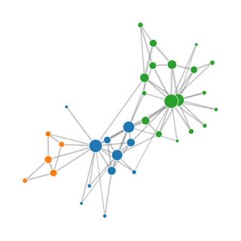
Fig. 2 Zachary’s karate club, coloured by the modules Infomap finds. The walker lingers inside each colour and crosses between them only rarely, which is exactly the structure the map equation compresses. The boundary nodes form a small extra module because naming it shortens the overall code.¶
API pointers¶
The codelength metrics this chapter defines all live on
Result: codelength,
one_level_codelength,
relative_codelength_savings, plus
num_top_modules and modules();
see Reading the result. infomap.run()
takes two_level=True for a flat partition, and steers the module count softly
with preferred_number_of_modules (carried via Options).
Going deeper¶
Source paper [Rosvall and Bergstrom, 2008]; a longer pedagogical account with the fast stochastic search algorithm [Rosvall et al., 2009].
The survey (§3) derives the map equation and compares it with modularity in depth [Smiljanić et al., 2026]; its companion notebook is
examples/notebooks/3.1 The two-level map equation.ipynb.