Incomplete data and regularization¶
Robustness
At a glance
When your network is missing links, standard Infomap overfits and splits nodes into many small spurious modules. The Bayesian regularized map equation adds a principled prior over transition rates so that only well-supported communities survive.
Missing links break the objective¶
Network data collected from real systems are almost always incomplete. A survey captures only a subset of acquaintances, and a citation database crawls only a fraction of references. When links are missing, the network is sparser than reality, and community detection methods that take the observed network at face value draw the wrong boundaries.
The standard map equation is prone to this. It minimises a Shannon entropy-based description length that systematically underestimates the true entropy when data are sparse [Basharin, 1959]. The bias grows as communities lose links, and the map equation’s two cost terms fall out of balance: the module codebooks look cheap to shrink, so the optimiser splits nodes into smaller and smaller groups, down to groups of two or three nodes with no principled support. Those modules are an artefact of noise.
The search algorithm and the number of trials are not the cause. The bias is in the objective itself: on sparse data it rewards splitting communities that the evidence does not support. The fix is a regularization mechanism built into the objective.
Regularization as a Bayesian prior¶
In the map equation, a community is a group of nodes where a random walker lingers (see The map equation). When the network is nearly complete, the observed degree of each node is a reliable estimate of how strongly it attracts the walker. When many links are missing, the observed degree is just a noisy sample of the true degree. Relying on that sample blindly inflates apparent differences between nodes, encourages the algorithm to draw boundaries around statistical accidents, and produces many tiny “communities” that would dissolve if you observed a few more links.
Regularization addresses this by blending what you observed with an uninformative prior: a featureless, fully-connected network with no community structure of its own.
The picture is similar to Bayesian smoothing for language models: a bigram count of zero does not mean two words never co-occur; you add a small pseudocount so the model is not overconfident about what it has not seen.
The regularized map equation¶
Smiljanić et al. [2020] introduced the regularized map equation for
undirected, unweighted networks; Smiljanić et al. [2021] extended it
to weighted and directed networks. Infomap implements both under the single
flag regularized=True.
Infomap’s prior network is the continuous configuration model: fully connected, with no community structure of its own. The random walker moves on the combination of it and the observed network — most steps follow observed links, but with a small, data-dependent probability the walker takes a prior step toward any node. Nodes with few observed links lean more on the prior; nodes with many links lean on their data. Where evidence is abundant, the data dominate and the prior barely matters. Where the network is sparse, the prior evens out the apparent cost differences that drive spurious splitting.
The strength of the prior is \(\lambda = C\,\ln N / N\), where \(N\) is the number of
nodes and \(C\) is the regularization_strength (default \(1\)). The value
\(\ln N / N\) is the edge probability at which an Erdős–Rényi random graph becomes
almost surely connected, which is what makes it a principled default (see the
toggle).
Why \(\lambda = \ln N / N\)
An Erdős–Rényi random graph on \(N\) nodes with edge probability \(\lambda\)
undergoes a connectivity phase transition at \(\lambda = \ln N / N\): below it the
graph almost surely breaks into isolated components, so a weaker prior cannot
stop the map equation from giving poorly-sampled nodes their own spurious
modules; above it the prior network is connected but still structureless, so it
adds no bias toward any grouping. The default \(C = 1\)
(regularization_strength=1.0) places the prior exactly at this critical point,
balancing resistance to overfitting against washing out real communities. Lower
values (e.g. \(C = 0.5\)) allow more communities; higher values push toward fewer.
For severely undersampled networks the regularized objective prefers the
one-module solution, reporting that the evidence does not support any community
structure.
A separate option, entropy_corrected, corrects the small-sample bias in the
entropy estimate itself; it is independent of the prior-network regularization
described here.
A 70%-sparse planted partition¶
The example below constructs a synthetic network with five planted communities of twelve nodes each: edges appear within communities with probability 0.7 and between communities with probability 0.02. It then removes 70 % of the edges uniformly at random to simulate incomplete observations.
Build the network¶
import networkx as nx
import infomap
import random

# Reproducible construction. We sample the planted-partition graph with Python's
# `random` rather than a library sampler, so the exact graph, and the module
# counts below, do not depend on the NumPy or NetworkX version.
random.seed(99)

n_communities = 5
n_per_community = 12
n = n_communities * n_per_community
community = {i: i // n_per_community for i in range(n)}

# Ground truth: 5 modules of 12 nodes. An edge forms within a community with
# probability 0.7 and between communities with probability 0.02.
g_full = nx.Graph()
g_full.add_nodes_from(range(n))
for i in range(n):
    for j in range(i + 1, n):
        p = 0.7 if community[i] == community[j] else 0.02
        if random.random() < p:
            g_full.add_edge(i, j)
print(f"Full graph : {g_full.number_of_nodes()} nodes, {g_full.number_of_edges()} edges")

# Remove 70 % of edges to simulate missing link observations.
edges = list(g_full.edges())
random.shuffle(edges)
removal_fraction = 0.70
g_sparse = g_full.copy()
g_sparse.remove_edges_from(edges[: int(removal_fraction * len(edges))])
print(f"Sparse graph: {g_sparse.number_of_nodes()} nodes, {g_sparse.number_of_edges()} edges")
print(f"({removal_fraction:.0%} of links removed)")
Full graph : 60 nodes, 255 edges
Sparse graph: 60 nodes, 77 edges
(70% of links removed)
Run standard vs. regularized Infomap¶
# Standard Infomap: no regularization
result_std = infomap.run(g_sparse, two_level=True, seed=99, num_trials=10)

# Regularized Infomap. We use regularization_strength=0.5 (gentler than the
# default 1.0, which over-regularizes this 70%-sparse graph toward one module).
result_reg = infomap.run(
    g_sparse,
    two_level=True,
    seed=99,
    num_trials=10,
    options=infomap.Options(regularized=True, regularization_strength=0.5),
)

modules_std = result_std.modules()
modules_reg = result_reg.modules()

print(f"Ground truth  : {n_communities} communities")
print(f"Standard      : {result_std.num_top_modules} modules  (codelength {result_std.codelength:.4f} bits/step)")
print(f"Regularized   : {result_reg.num_top_modules} modules  (codelength {result_reg.codelength:.4f} bits/step)")
Ground truth  : 5 communities
Standard      : 14 modules  (codelength 3.8976 bits/step)
Regularized   : 7 modules  (codelength 5.6441 bits/step)
On this 70 %-sparse graph standard Infomap over-partitions: it reports many more
modules than the five planted communities (see the counts above), because the
objective underestimates the true description length on a sparse graph and
commits to a finer partition than the data warrant. Regularization merges the
noise-driven splits and pulls the count back toward five. It does not always land
exactly on the ground truth, and at this severe sparsity the principled default
regularization_strength=1.0 over-regularizes, collapsing toward a single
module, which is why this example uses a gentler 0.5.
Module size distributions
The spurious modules standard Infomap adds are small groups of nodes that lost most of their links through random removal, leaving them weakly connected to any community. Regularization treats those nodes as part of the nearest genuine module because the prior pseudocounts smooth out the sparse links.
Visualise the regularized partition¶
import matplotlib.pyplot as plt
from myst_nb import glue

from docs_viz import draw_partition

flow = {n.node_id: n.flow for n in result_reg.nodes()}
fig = draw_partition(g_sparse, modules_reg, flow=flow)
glue("fig-incomplete-data", fig, display=False)
plt.close(fig)
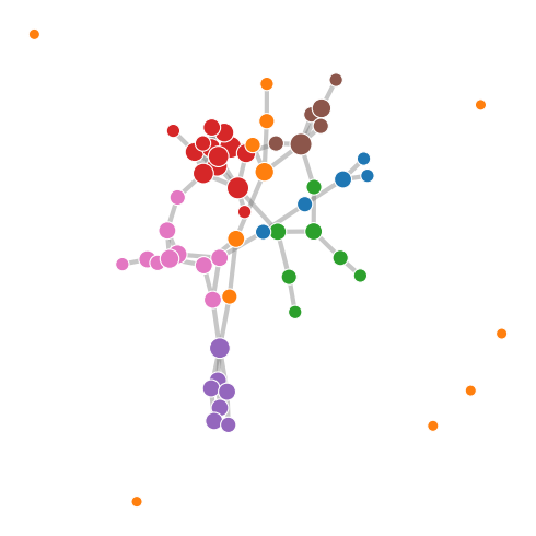
Fig. 15 A sparse network partitioned with the regularized map equation (regularized=True). The Bayesian prior keeps weakly-sampled nodes in larger modules instead of breaking them into noise-driven singletons.¶
Each colour is one regularized module. Even with most links removed, the regularized run recovers far fewer, larger modules than the unregularized one, close to the planted five.
API pointers¶
infomap.run()withoptions=Options(regularized=True)activates the Bayesian regularized map equation;regularization_strength(the constant \(C\) above, default1.0) tunes the prior. It applies to undirected, weighted, and directed networks ([Smiljanić et al., 2020]; [Smiljanić et al., 2021]).Run metrics —
codelength(Bayesian-corrected under regularization),num_top_modules,modules()— are covered in Reading the result.
Going deeper¶
Source papers: the regularized map equation on undirected, unweighted networks [Smiljanić et al., 2020], and its extension to weighted and directed networks via an empirical Bayes estimate of transition rates [Smiljanić et al., 2021].
Module-level reliability scores that tell a robust partition from one driven by sampling noise [Neuman et al., 2025].
The survey (§7) sets incomplete data, overfitting, and the regularized map equation in context [Smiljanić et al., 2026]; its companion notebook
examples/notebooks/7 Networks with incomplete data.ipynbruns link-removal experiments with cross-validation.