Running Infomap¶
How-to
At a glance
Most runs need only a seed, a num_trials count, and perhaps a flow-model
choice such as directed. The rest of Infomap’s options split into flow-model
settings, which define the random walk, and search settings, which control how
hard Infomap looks.
Add two_level if you want a flat partition instead of the multilevel default.
The shortest useful run:
import networkx as nx
import infomap

result = infomap.run(
    nx.karate_club_graph(),
    seed=123,        # reproducible
    num_trials=10,   # keep the best of 10 restarts
    two_level=True,  # flat partition; omit for the multilevel default
)
print(result.num_top_modules, result.codelength)
Everything below is when and why to reach for the other options. For the why behind the flow model itself, see Concepts.
Two kinds of options¶
Infomap has dozens of options, but they fall into two groups:
Flow-model options (
directed,markov_time,teleportation_probability) change how the random walk is defined. They encode your beliefs about the system; the wrong choice gives a partition that scores well but means little.Search options (
seed,num_trials,converge) change how hard the search works, not which partition Infomap looks for. They only affect how reliably the stochastic search finds the optimum [Calatayud et al., 2019].
The theory behind them lives in Concepts: Flow and random walks for flow and teleportation, Hierarchy and the multilevel map equation and Reading Infomap through Louvain and Leiden for resolution, and Incomplete data and regularization for regularization.
The options, one task each¶
Each option below comes with a small graph you can run as you read.
Setting up¶
import networkx as nx
import infomap
import random

# ── Helper: build an 8-clique ring (clear, clean structure) ──────────────────
G_ring = nx.ring_of_cliques(8, 5)   # 8 cliques × 5 nodes = 40 nodes

# ── Helper: build a weakly-structured graph (noisy, degenerate landscape) ───
def make_weak_structure(n_communities=6, n_per=8, p_in=0.55, p_out=0.08, seed=123):
    """Planted-partition graph with intentionally weak community signal."""
    rng = random.Random(seed)
    G = nx.Graph()
    n = n_communities * n_per
    G.add_nodes_from(range(n))
    for i in range(n):
        for j in range(i + 1, n):
            ci, cj = i // n_per, j // n_per
            p = p_in if ci == cj else p_out
            if rng.random() < p:
                G.add_edge(i, j)
    return G

G_noisy = make_weak_structure()
print(f"Ring of cliques: {G_ring.number_of_nodes()} nodes, {G_ring.number_of_edges()} edges")
print(f"Weak structure:  {G_noisy.number_of_nodes()} nodes, {G_noisy.number_of_edges()} edges")
Ring of cliques: 40 nodes, 88 edges
Weak structure:  48 nodes, 175 edges
seed and reproducibility¶
seed fixes the internal random number generator. With the same seed you get
the same partition on every run, which makes results shareable and publishable.
The default seed=123 is reproducible too, but setting the seed yourself ties
each result to the code that produced it.
# Two runs with the same seed produce the same partition.
for attempt in range(2):
    result = infomap.run(G_ring, two_level=True, seed=123, num_trials=10)
    print(f"Run {attempt + 1}: modules={result.num_top_modules}, L={result.codelength:.4f}")
Run 1: modules=8, L=3.0373
Run 2: modules=8, L=3.0373
num_trials and solution quality¶
A single trial can get trapped in a local minimum. On graphs with clear, distinct communities, like the ring of cliques, this rarely matters because most starting points converge to the same solution. On a noisy or ambiguous graph the landscape has many near-degenerate minima, and a single trial is unreliable.
# On the noisy graph, different seeds land in different local minima.
print("Single trial (num_trials=1), five different seeds:")
for seed in [1, 7, 42, 99, 123]:
    result = infomap.run(G_noisy, two_level=True, seed=seed, num_trials=1)
    print(f"  seed={seed}: L={result.codelength:.4f}, modules={result.num_top_modules}")
Single trial (num_trials=1), five different seeds:
  seed=1: L=5.4912, modules=4
  seed=7: L=5.4326, modules=5
  seed=42: L=5.4538, modules=5
  seed=99: L=5.4352, modules=5
  seed=123: L=5.5043, modules=1
# More trials explore more of the landscape and find a lower, stable minimum.
print("Fixed seed=123, varying num_trials:")
for num_trials in [1, 5, 20]:
    result = infomap.run(G_noisy, two_level=True, seed=123, num_trials=num_trials)
    print(f"  num_trials={num_trials:2d}: L={result.codelength:.4f}, modules={result.num_top_modules}")
Fixed seed=123, varying num_trials:
  num_trials= 1: L=5.5043, modules=1
  num_trials= 5: L=5.4326, modules=5
  num_trials=20: L=5.4326, modules=5
Here the single trial with seed=123 lands at a higher codelength (worse
minimum) than num_trials=20 with the same seed: a single trial can settle in a
local trap, and the extra trials find a partition that compresses the random
walk more efficiently. Which single trial gets stuck depends on the seed, so
the gap is not guaranteed for any particular seed. The codelength converges:
once you are reliably in the deepest valley, adding more trials does not change
the answer [Calatayud et al., 2019].
Rule of thumb. Use num_trials=1 for quick exploration. Use
num_trials=10 for most analyses. Use num_trials=20 or more (up to around
50, or converge=True with a higher cap) when you need high confidence in
the global minimum, when you are comparing partitions across networks, or on
networks with weak or diffuse community structure.
converge
converge=True treats num_trials as a cap and stops early once the best
codelength has stopped improving. This gives you “as many trials as you need
but no more,” which is useful when you are unsure how many trials your network
requires. It is not one of the five common keywords, so carry it via Options:
infomap.run(graph, options=Options(converge=True), num_trials=50).
two_level versus multilevel¶
By default Infomap finds a hierarchical partition with as many levels as the
flow supports. Each level is a coarser view of the same structure.
two_level=True forces a single flat partition, which helps when you know your
network is not hierarchical, or when you need a simple cluster assignment for
downstream analysis.
# Build a graph with genuine nested hierarchy:
# 2 top groups → 2 subgroups each → 2 cliques of 5 nodes
# Edge weights shrink at each scale, creating clear nesting.
def hierarchical_graph():
    G = nx.Graph()
    nid = 0
    top_groups = []
    for _ in range(2):
        subgroups = []
        for _ in range(2):
            cliques = []
            for _ in range(2):
                members = list(range(nid, nid + 5))
                nid += 5
                for i in range(len(members)):
                    for j in range(i + 1, len(members)):
                        G.add_edge(members[i], members[j], weight=100.0)
                cliques.append(members)
            G.add_edge(cliques[0][0], cliques[1][0], weight=10.0)
            subgroups.append(cliques)
        G.add_edge(subgroups[0][0][0], subgroups[1][0][0], weight=1.0)
        top_groups.append(subgroups)
    G.add_edge(top_groups[0][0][0][0], top_groups[1][0][0][0], weight=0.1)
    return G

G_hier = hierarchical_graph()

for two_level in [False, True]:
    result = infomap.run(G_hier, two_level=two_level, seed=123, num_trials=10)

    m_top = result.modules(depth=1)    # top-level groups
    m_leaf = result.modules(depth=-1)  # finest-level assignments

    print(f"two_level={two_level}:")
    print(f"  levels={result.num_levels}, top modules={result.num_top_modules}")
    print(f"  distinct groups at depth 1:      {len(set(m_top.values()))}")
    print(f"  distinct groups at finest level: {len(set(m_leaf.values()))}")
    print(f"  L={result.codelength:.4f}")
two_level=False:
  levels=4, top modules=2
  distinct groups at depth 1:      2
  distinct groups at finest level: 8
  L=2.3762
two_level=True:
  levels=2, top modules=8
  distinct groups at depth 1:      8
  distinct groups at finest level: 8
  L=2.3848
With two_level=False, the multilevel solution recovers the built-in nesting:
the two main branches at the top and the eight cliques at the finest level,
reached with result.modules(depth=-1) (the cell above prints the exact counts).
The codelength is lower because the deeper code captures the real hierarchy. With
two_level=True, the eight cliques become the top-level modules and the nested
structure is invisible.
Use result.modules(depth=k) to access any level of the hierarchy. The default
result.modules() returns level 1, the coarsest (top modules); pass depth=-1
for the finest (leaf) level.
directed and the flow model¶
When your links represent directed flow (citations, hyperlinks, metabolic
reactions, transit routes), directed=True tells Infomap to use the
directionality to define the random walk. The walker follows links in their
stated direction, and unrecorded teleportation keeps the walk ergodic. Ignoring
direction on the same graph often misses the real community structure, because
it treats every link as symmetric.
# A directed graph: three directed cliques connected by directed bridges.
# The directed structure groups nodes by which clique's flow they participate in.
G_dir = nx.DiGraph()
# Three directed cliques
for offset in [0, 4, 8]:
    nodes = list(range(offset, offset + 4))
    for u in nodes:
        for v in nodes:
            if u != v:
                G_dir.add_edge(u, v)
# Directed bridges forming an outer loop
G_dir.add_edge(3, 4)
G_dir.add_edge(7, 8)
G_dir.add_edge(11, 0)

print(f"Directed graph: {G_dir.number_of_nodes()} nodes, {G_dir.number_of_edges()} edges")

for directed in [False, True]:
    result = infomap.run(G_dir, directed=directed, two_level=True,
                         seed=123, num_trials=10)
    print(f"directed={directed}: modules={result.num_top_modules}, L={result.codelength:.4f}")
Directed graph: 12 nodes, 39 edges
directed=False: modules=3, L=2.5174
directed=True: modules=3, L=2.4468
Both settings recover three modules here because the graph is strongly clustered. On noisier real-world directed networks the difference is more pronounced: the directed walk respects asymmetric flow and tends to find tighter modules corresponding to true circulation patterns.
Teleportation probability. teleportation_probability (\(\tau\)) sets the
random-surfer teleportation rate; the default 0.15 is rarely worth changing.
See Flow and random walks for why unrecorded teleportation makes
the partition robust to \(\tau\).
markov_time as a resolution dial¶
The map equation operates at the natural timescale of one random-walk step.
markov_time shifts this timescale: values below 1 encode the walk more
frequently (favouring more, smaller modules) and values above 1 encode it less
frequently (favouring fewer, larger modules). This is the principled way to
examine structure at a specific resolution when the data does not have a natural
scale [Kheirkhahzadeh et al., 2016].
# The ring of cliques has 8 genuine cliques. markov_time merges them
# into larger clusters as it increases, giving a resolution sweep.
print("markov_time sweep on a ring of 8 cliques (5 nodes each):")
print(f"  graph: {G_ring.number_of_nodes()} nodes, {G_ring.number_of_edges()} edges")
print()

for mt in [0.5, 1.0, 2.0, 4.0, 8.0]:
    result = infomap.run(G_ring, two_level=True, markov_time=mt,
                         seed=123, num_trials=10)
    print(f"  markov_time={mt:.1f}: {result.num_top_modules} modules")
markov_time sweep on a ring of 8 cliques (5 nodes each):
  graph: 40 nodes, 88 edges

  markov_time=0.5: 8 modules
  markov_time=1.0: 8 modules
  markov_time=2.0: 8 modules
  markov_time=4.0: 4 modules
  markov_time=8.0: 3 modules
At markov_time=1.0 (the default) Infomap recovers all 8 cliques. As the
Markov time grows, smaller modules become too expensive to maintain and adjacent
cliques merge. This gives you a natural scale sweep without changing the network.
The multilevel map equation is usually the better first choice [Kawamoto and Rosvall, 2015]: it finds scale automatically and has a less restrictive
resolution limit than the two-level version. Use markov_time when you
specifically want to study structure at a given scale, or when reviewers ask
“what happens at a coarser resolution?”
regularized for sparse data¶
Setting regularized=True (carried via Options, as in the loop below) enables
the Bayesian regularized map equation for sparse or
incompletely sampled networks, and regularization_strength scales the prior
(higher merges more modules); see Incomplete data and regularization for why
sparse data over-split and how the prior fixes it. On a graph as small as the
karate club the prior quickly overwhelms the data:
# On the small karate club the regularization prior competes with the data:
# at half strength the three modules survive, and at the default strength
# the prior already outweighs the data and collapses them into one.
G_karate = nx.karate_club_graph()

for label, options in [
    ("baseline",                  infomap.Options()),
    ("regularized, strength=0.5", infomap.Options(regularized=True, regularization_strength=0.5)),
    ("regularized (default 1.0)", infomap.Options(regularized=True)),
]:
    result = infomap.run(G_karate, options=options, two_level=True, seed=123, num_trials=10)
    print(f"{label}: modules={result.num_top_modules}, L={result.codelength:.4f}")
baseline: modules=3, L=4.0874
regularized, strength=0.5: modules=3, L=4.7197
regularized (default 1.0): modules=1, L=4.8780
The default strength already merges everything on a network this small. For a worked example on a sparsely sampled planted partition, see Incomplete data and regularization.
Why trials matter, visualised¶
A picture of the effect: run the noisy graph once per seed with a single trial, and compare those codelengths against the lowest a longer search finds.
import matplotlib.pyplot as plt
from myst_nb import glue

# Codelength from one trial per seed ...
single_L = []
for s in range(1, 13):
    single_L.append(
        infomap.run(G_noisy, two_level=True, seed=s, num_trials=1).codelength
    )

# ... versus the lowest codelength a longer search finds. Several seeds at 50
# trials each, so the reference is the best partition rather than one lucky (or
# unlucky) run; take the floor of everything shown so the line is a true minimum.
best_L = min(
    infomap.run(G_noisy, two_level=True, seed=s, num_trials=50).codelength
    for s in (1, 42, 123)
)
best_L = min([best_L, *single_L])

fig, ax = plt.subplots(figsize=(6, 3.2))
ax.scatter(range(1, len(single_L) + 1), single_L,
           color="0.45", zorder=3, label="single trial (num_trials=1)")
ax.axhline(best_L, color="tab:blue", lw=2, label=f"lowest codelength found = {best_L:.3f}")
ax.set_xlabel("seed")
ax.set_ylabel("codelength (bits/step)")
ax.legend(loc="best", fontsize=8)
fig.tight_layout()
glue("fig-running-and-options", fig, display=False)
plt.close(fig)
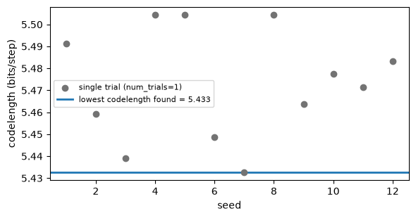
Fig. 6 Each grey point is one trial’s codelength for a different seed, scattered widely. A single trial rarely reaches the best partition Infomap can find (blue line) — most settle in a worse local minimum. Running more trials and keeping the lowest codelength is what gets you there; here only seed 7 finds it in one trial.¶
Reusable configuration¶
When you run several networks with the same settings, capture them once as an
Options and pass the instance to each run. Keyword overrides on
the call still take precedence:
from infomap import Options

options = Options(two_level=True, seed=123, num_trials=10)
for name, graph in [("ring of cliques", G_ring), ("karate club", G_karate)]:
    result = infomap.run(graph, options=options)
    print(f"{name}: {result.num_top_modules} modules, L={result.codelength:.4f}")
ring of cliques: 8 modules, L=3.0373
karate club: 3 modules, L=4.0874
Pitfalls¶
No whitespace in paths or names. Options reach the engine as one whitespace-separated argument string, which has no quoting, so a value containing a space cannot survive the trip. Infomap rejects such a value rather than truncating it:
cluster_data="my file.clu"raisesValueError. Rename the file, or point at it from a directory whose path has no spaces. This is a limitation of the engine boundary, not of the Python API — the same holds for the R and JavaScript bindings and for the command line.seed=0raises. Infomap requiresseed >= 1; use any positive integer.Codelengths are not comparable across
meta_data_ratevalues.result.codelengthreports the combined objective, the topological term plus the weighted attribute term, so it rises with the rate even when the partition does not change (see Networks with metadata).More trials never hurt correctness, only runtime. If repeated runs disagree, raise
num_trials(or cap trials withoptions=Options(converge=True)) rather than trusting one fit.Sparse or under-sampled data over-splits. Reach for
options=Options(regularized=True)(see Incomplete data and regularization).
API pointers¶
Options is the canonical option carrier: infomap.run()
and infomap.Network.run() both take options=. On the stateful
infomap.Infomap the advanced keywords stay accepted but are
pending-deprecated and leave the signature in 3.0 (Deprecation policy).
After a run, metrics and partition accessors live on the returned
Result (Reading the result).
The most-used options — all fields of Options, with the five
common ones also accepted directly on infomap.run():
Option |
Type |
Default |
What it controls |
|---|---|---|---|
|
int |
123 |
RNG seed; must be ≥ 1 |
|
int |
1 |
Independent restarts; keep the best |
|
bool |
False |
Stop early when codelength plateaus |
|
bool |
False |
Force a flat (non-hierarchical) partition |
|
bool |
None |
Respect link direction |
|
float |
0.15 |
\(\tau\) in the random-surfer model |
|
bool |
False |
Include teleportation in flow encoding |
|
float |
1.0 |
Resolution scale |
|
bool |
False |
Bayesian regularization for sparse data |
|
float |
1.0 |
How strongly to regularize |
For the full set of options as a searchable table, see the
Options reference in the API reference.
Routing the engine log through Python logging¶
The Python API is quiet by default. When you do want the engine’s progress log — in a notebook, application logs, or a file — one line opts in:
import infomap

infomap.enable_log()

result = infomap.run([(1, 2), (1, 3), (2, 3), (3, 4), (4, 5), (4, 6), (5, 6)])

infomap.disable_log()
print(f"Found {result.num_top_modules} modules")
Infomap v2.15.1
started 2026-08-04 09:08:34
- Input
- Output disabled
- Runtime OpenMP 201511 with 4 threads
Flow
Model undirected
Method undirected links
Node flow sum 1
Link flow sum 1
Threads
CPUs available 4
Thread budget 4 (cpuset)
Inner parallelization disabled
Trial 1/1 started 2026-08-04 09:08:34
Optimization
- Two-level 9.23%, 0% -> codelength 2.320730357, 2 modules
- Super-level 0% -> codelength 2.320730357, 2 top modules
- Recursive 0% -> 2 levels, codelength 2.320730357
Done trial 1/1 in 0.007838004s | codelength 2.320730357
Summary after 1 trial
Nodes 6
Links 7
Average degree 2.3
Top modules 2 (2 non-trivial)
Levels 2
One-level codelength 2.556656707
Best codelength 2.320730357
Relative savings 9.23%
Levels
Level Modules Leaves Avg children Module bits Leaf bits Total bits
1 2 0 2.00 0.142857 0.000000 0.142857
2 0 6 3.00 0.000000 2.177873 2.177873
Total 2 6 2.75 0.142857 2.177873 2.320730
Finished 2026-08-04 09:08:34 in 0.0245269s
Found 2 modules
enable_log() attaches a plain handler to the standard
"infomap" logger; that is all the opt-in is. For full control — formats,
files, your logging pipeline — skip the helper and configure the logger with
standard logging; any handler attached directly to it engages the same
routing:
import logging

logging.getLogger("infomap").addHandler(my_handler)
logging.getLogger("infomap").setLevel(logging.INFO)
enable_log() (above) is the supported way to see the engine log;
the silent= and verbosity_level= keywords are pending-deprecated and leave
the API in 3.0. One timing nuance if you route through logging: a stateful
Infomap bakes its silence in at construction, so configure
logging before you build one (its runs warn otherwise), whereas the one-shot
infomap.run() always respects the current configuration.
Network engines stay silent for their whole lifetime (see
Network.run).
Going deeper¶
The options guide notebook lists every option in a searchable table, generated from the installed package so it matches your version. Start here for the exhaustive reference.
The survey (§4) covers method selection and the flow-model justification [Smiljanić et al., 2026].
The quantitative case for multiple trials [Calatayud et al., 2019].
Why unrecorded teleportation produces robust directed partitions [Lambiotte and Rosvall, 2012].
Why the map equation’s resolution limit is less restrictive than modularity’s [Kawamoto and Rosvall, 2015].
The Markov-time mechanism and its efficient resolution sweeps [Kheirkhahzadeh et al., 2016].