Compare Infomap and Leiden in a Scanpy workflow

Run Infomap on an AnnData neighbor graph and compare it with Scanpy’s Leiden workflow. The example uses a small synthetic dataset, so it needs no downloads and stays reproducible.

Infomap reads the sparse observation graph from adata.obsp and writes categorical labels to adata.obs, matching Scanpy tl conventions. Leiden is the standard Scanpy baseline shown here.

from importlib.metadata import version
import warnings

import infomap
import pandas as pd
from sklearn.datasets import make_blobs

# import scanpy after filterwarnings so its import-time warning stays silenced
warnings.filterwarnings("ignore", message="IProgress not found.*")
import scanpy as sc  # noqa: E402

print("infomap:", infomap.__version__)
print("scanpy:", version("scanpy"))
print("pandas:", pd.__version__)

infomap: 2.13.0
scanpy: 1.12.1
pandas: 2.3.3

Create a small AnnData object

The dataset is synthetic and local. Scanpy builds a nearest-neighbor graph in adata.obsp["connectivities"], which is the same graph used by Scanpy clustering tools and the default graph read by infomap.tl.infomap().

X, truth = make_blobs(
    n_samples=120,
    centers=4,
    n_features=12,
    cluster_std=1.8,
    random_state=123,
)
adata = sc.AnnData(X)
adata.obs["truth"] = pd.Categorical([str(label) for label in truth])

sc.pp.neighbors(adata, n_neighbors=12, random_state=123)
sc.tl.umap(adata, random_state=123)

adata

AnnData object with n_obs × n_vars = 120 × 12
    obs: 'truth'
    uns: 'neighbors', 'umap'
    obsm: 'X_umap'
    obsp: 'distances', 'connectivities'

Run Infomap and Leiden

infomap.tl.infomap() stores labels in adata.obs[key_added] and run metadata in adata.uns[key_added]. Scanpy’s Leiden function is called with the same neighbor graph.

infomap.tl.infomap(
    adata,
    key_added="infomap",
    seed=123,
    num_trials=20,
)

sc.tl.leiden(
    adata,
    key_added="leiden",
    random_state=123,
    flavor="igraph",
    n_iterations=2,
    directed=False,
)

print("Infomap communities:", adata.obs["infomap"].nunique())
print("Leiden communities:", adata.obs["leiden"].nunique())

adata.uns["infomap"]

Infomap communities: 4
Leiden communities: 4

{'params': {'directed': False,
  'use_weights': True,
  'neighbors_key': None,
  'obsp': 'connectivities',
  'args': None,
  'silent': True,
  'no_file_output': True,
  'seed': 123,
  'num_trials': 20},
 'n_modules': 4,
 'codelength': 4.832376351710865}

Compare assignments

The labels are categorical strings because that is the common Scanpy representation for cluster assignments.

comparison = adata.obs[["truth", "infomap", "leiden"]].copy()
comparison.head(10)

	truth	infomap	leiden
0	0	1	0
1	2	2	1
2	0	1	0
3	3	3	2
4	3	3	2
5	2	2	1
6	0	1	0
7	2	2	1
8	3	3	2
9	3	3	2

from sklearn.metrics import adjusted_mutual_info_score, normalized_mutual_info_score

metrics = pd.DataFrame(
    [
        {
            "method": "infomap",
            "AMI vs truth": adjusted_mutual_info_score(
                comparison["truth"], comparison["infomap"]
            ),
            "NMI vs truth": normalized_mutual_info_score(
                comparison["truth"], comparison["infomap"]
            ),
        },
        {
            "method": "leiden",
            "AMI vs truth": adjusted_mutual_info_score(
                comparison["truth"], comparison["leiden"]
            ),
            "NMI vs truth": normalized_mutual_info_score(
                comparison["truth"], comparison["leiden"]
            ),
        },
    ]
)
metrics

	method	AMI vs truth	NMI vs truth
0	infomap	1.0	1.0
1	leiden	1.0	1.0

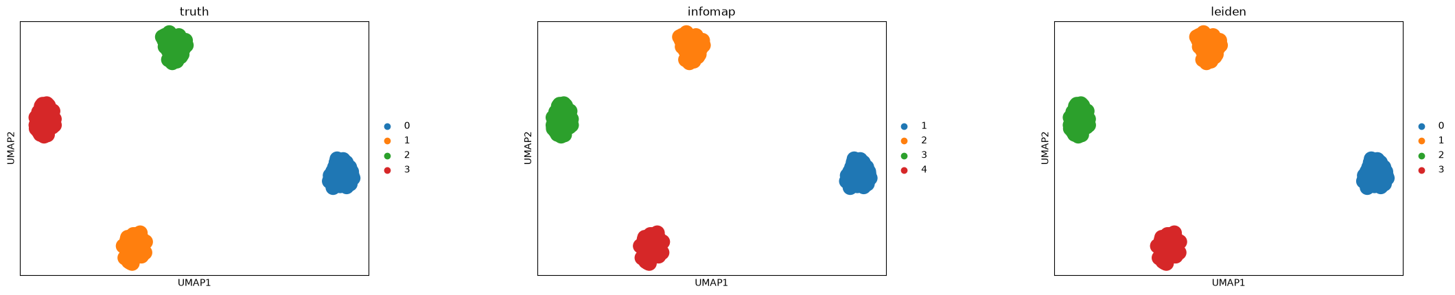
Visualize the clusters

Color the same UMAP layout by the known synthetic labels and the detected communities.

sc.pl.umap(adata, color=["truth", "infomap", "leiden"], wspace=0.35)

Notes on graph choices

By default, Infomap uses adata.obsp["connectivities"]. Pass neighbors_key when using a named Scanpy neighbor graph, or obsp/adjacency when selecting a graph. Use directed=True for directed observation graphs and use_weights=False for unweighted treatment of nonzero sparse entries.

Citation and further reading

If you use Infomap in published work, mapequation.org recommends citing two things: the map equation paper (Rosvall and Bergstrom, 2008, https://doi.org/10.1073/pnas.0706851105) for the method, and the MapEquation software package (Edler, Holmgren, and Rosvall) for the implementation and version. See How to cite for BibTeX.

See also the quickstart for a first run and the options guide for the parameters used here.