Compare Infomap and Louvain with NetworkX

Run Infomap next to Louvain in a NetworkX workflow. The example uses Zachary’s karate club graph: small, built into NetworkX, and a community-detection staple.

Infomap optimizes the map equation: it searches for a partition that compresses the description of flow on the network. Louvain optimizes modularity. The goal here is not to declare a universal winner, but to make the outputs easy to run, inspect, compare, visualize, and export.

from pathlib import Path

import infomap
import matplotlib.pyplot as plt
import networkx as nx
import pandas as pd

print("infomap:", infomap.__version__)
print("networkx:", nx.__version__)
print("pandas:", pd.__version__)

infomap: 2.13.0
networkx: 3.6.1
pandas: 2.3.3

Load a small graph

nx.karate_club_graph() is undirected and unweighted. For weighted graphs, pass the edge attribute name with weight="weight"; for unweighted graphs, pass weight=None. Infomap detects directed NetworkX graphs automatically when the input is a DiGraph.

graph = nx.karate_club_graph()
nodes = list(graph.nodes())
print(graph)
print("nodes:", graph.number_of_nodes())
print("edges:", graph.number_of_edges())

Graph named "Zachary's Karate Club" with 34 nodes and 78 edges
nodes: 34
edges: 78

Run the community methods

infomap.find_communities() follows the NetworkX convention of returning a partition as list[set] while preserving the original node labels. NetworkX provides Louvain through nx.community.louvain_communities().

def partition_to_labels(partition, ordered_nodes):
    labels = {}
    for community_id, community in enumerate(partition, start=1):
        for node in community:
            labels[node] = community_id
    return [labels[node] for node in ordered_nodes]


infomap_partition = infomap.find_communities(
    graph,
    weight=None,
    seed=123,
    num_trials=20,
)

louvain_partition = nx.community.louvain_communities(
    graph,
    weight=None,
    seed=123,
)

print("Infomap communities:", len(infomap_partition))
print("Louvain communities:", len(louvain_partition))

Infomap communities: 3
Louvain communities: 4

Compare assignments

Community IDs are local labels. Their numeric values only identify groups within one result; they should not be interpreted as stable or ordered labels across methods.

df = pd.DataFrame(
    {
        "node": nodes,
        "club": [graph.nodes[node]["club"] for node in nodes],
        "infomap": partition_to_labels(infomap_partition, nodes),
        "louvain": partition_to_labels(louvain_partition, nodes),
    }
)

df.head(10)

	node	club	infomap	louvain
0	0	Mr. Hi	1	1
1	1	Mr. Hi	1	1
2	2	Mr. Hi	1	1
3	3	Mr. Hi	1	1
4	4	Mr. Hi	2	2
5	5	Mr. Hi	2	2
6	6	Mr. Hi	2	2
7	7	Mr. Hi	1	1
8	8	Mr. Hi	3	4
9	9	Officer	1	4

summary = df.drop(columns="node").nunique().rename("communities").to_frame()
summary

	communities
club	2
infomap	3
louvain	4

Simple similarity metrics

Adjusted mutual information (AMI) and normalized mutual information (NMI) compare each detected assignment with the known karate-club split. They are useful checks, but they do not replace inspecting the graph and understanding the objective each method optimizes.

from sklearn.metrics import adjusted_mutual_info_score, normalized_mutual_info_score

metrics = pd.DataFrame(
    [
        {
            "method": "infomap",
            "AMI vs truth": adjusted_mutual_info_score(df["club"], df["infomap"]),
            "NMI vs truth": normalized_mutual_info_score(df["club"], df["infomap"]),
        },
        {
            "method": "louvain",
            "AMI vs truth": adjusted_mutual_info_score(df["club"], df["louvain"]),
            "NMI vs truth": normalized_mutual_info_score(df["club"], df["louvain"]),
        },
    ]
)
metrics

	method	AMI vs truth	NMI vs truth
0	infomap	0.551082	0.56838
1	louvain	0.566666	0.58785

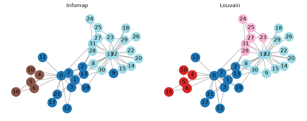
Visualize the partitions

The same layout is reused for each method so the visual comparison focuses on module assignments rather than node placement.

methods = ["infomap", "louvain"]
pos = nx.spring_layout(graph, seed=123)
fig, axes = plt.subplots(1, len(methods), figsize=(5 * len(methods), 4), squeeze=False)

for ax, method in zip(axes[0], methods):
    colors = [df.loc[df["node"] == node, method].iloc[0] for node in graph.nodes]
    nx.draw_networkx(
        graph,
        pos=pos,
        node_color=colors,
        cmap="tab20",
        with_labels=True,
        node_size=450,
        edge_color="#999999",
        ax=ax,
    )
    ax.set_title(method.title())
    ax.axis("off")

plt.tight_layout()

Export Infomap results

For downstream tools, write Infomap module IDs back to the NetworkX graph and export with NetworkX’s GraphML or GEXF writers. The export helpers can also add hierarchical Infomap attributes when you need more than top-level modules.

export_graph = graph.copy()
infomap.find_communities(
    export_graph,
    weight=None,
    module_attribute="infomap",
    flow_attribute="infomap_flow",
    seed=123,
    num_trials=20,
)

export_dir = Path("output")
export_dir.mkdir(exist_ok=True)
graphml_path = export_dir / "karate-infomap.graphml"
gexf_path = export_dir / "karate-infomap.gexf"

nx.write_graphml(export_graph, graphml_path)
nx.write_gexf(export_graph, gexf_path)
print("wrote:", graphml_path)
print("wrote:", gexf_path)

pd.DataFrame.from_dict(dict(export_graph.nodes(data=True)), orient="index").head()

wrote: output/karate-infomap.graphml
wrote: output/karate-infomap.gexf

	club	infomap	infomap_flow
0	Mr. Hi	1	0.102564
1	Mr. Hi	1	0.057692
2	Mr. Hi	1	0.064103
3	Mr. Hi	1	0.038462
4	Mr. Hi	2	0.019231

Citation and further reading

If you use Infomap in published work, mapequation.org recommends citing two things: the map equation paper (Rosvall and Bergstrom, 2008, https://doi.org/10.1073/pnas.0706851105) for the method, and the MapEquation software package (Edler, Holmgren, and Rosvall) for the implementation and version. See How to cite for BibTeX.

See also the quickstart for a first run, the options guide for the parameters used here, and compare-infomap-louvain-leiden-igraph for the same comparison with igraph-native clustering objects.